
How an end-to-end MLOps pipeline actually works
A journey from machine learning experiment to live production application, and the playbook for product managers to bridge the gap between data science and deployment.

Many thanks to my MLOps professor at Sorbonne University, Kamila Kare, for his excellent course and for suggesting this very project.
Content
From a data science lab to a live feature
Picture this. You’re grabbing a coffee, and a data scientist from your team rushes over, laptop in hand, absolutely beaming. “I’ve got it!” they say, showing you a screen full of code, charts, and notes. This is their digital lab, a tool often called a Python or Jupyter Notebook, where they mix code and data to experiment, test theories, and invent. It’s where the magic happens.
But an engine on a test bench isn’t a car on the road. The gap between a model that works in the lab and a feature that works reliably in the hands of thousands of users, what I call the “factory,” is massive and filled with hidden risks.
For a long time, I felt like I was managing from the other side of that gap, responsible for a technical “black box” without the vocabulary to ask the right questions. That feeling became my motivation. I realized that to lead AI products effectively, I didn’t need to become a coder, but I had to understand the factory floor. So, I went down the MLOps rabbit hole and decided to build a real, end-to-end system to see how all the pieces fit together.
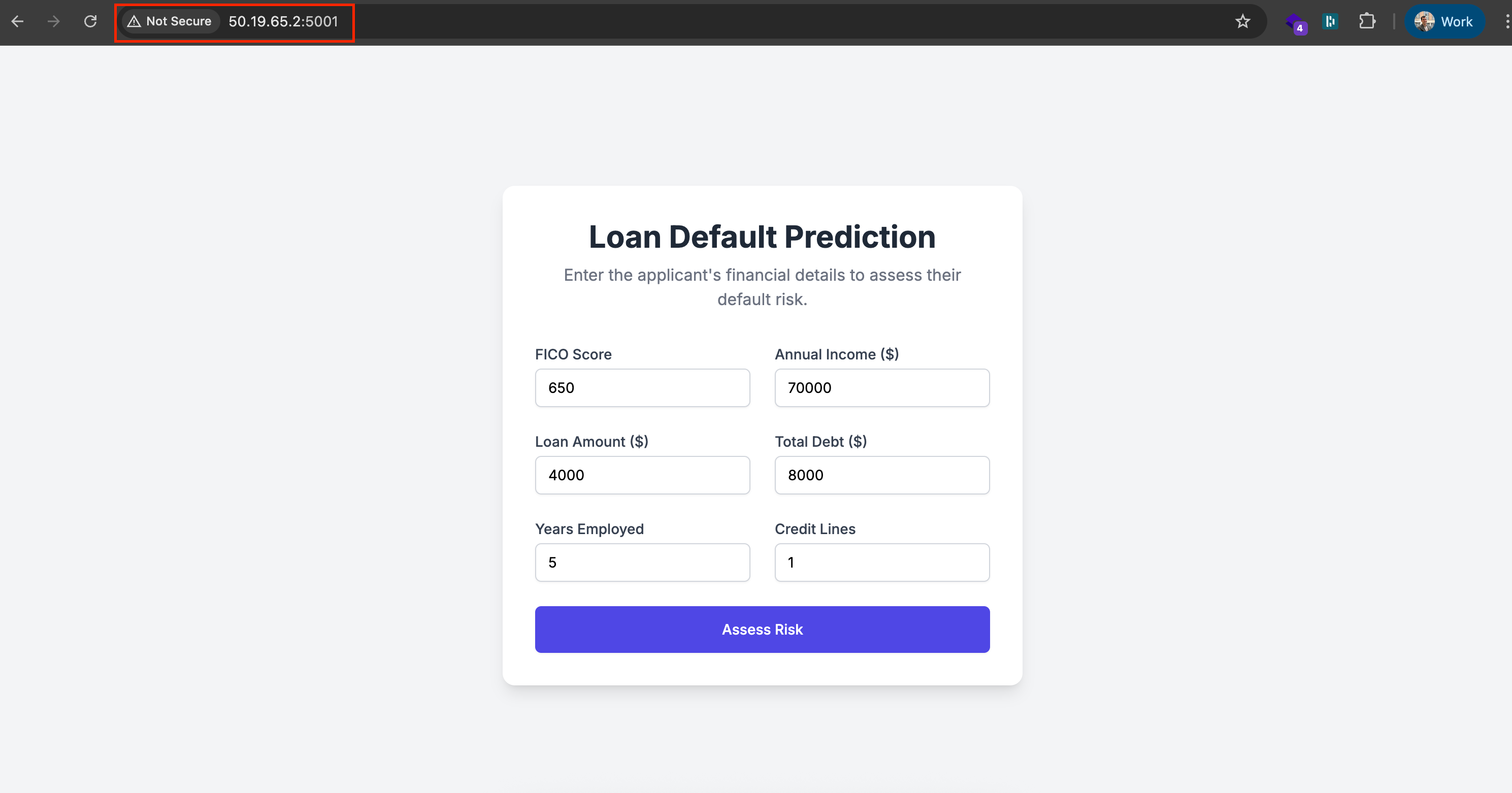
The result is a simple web app that predicts the probability of a customer defaulting on a loan, but more importantly, it’s backed by a fully automated MLOps pipeline that takes it from code on my machine to a live service in the cloud.
This article is the playbook I wish I had when I started. My goal is to give you a clear framework and a shared language to bridge that gap between data science and deployment. We’ll demystify the jargon and walk through the entire journey, turning that technical black box into a transparent assembly line you can manage with confidence.
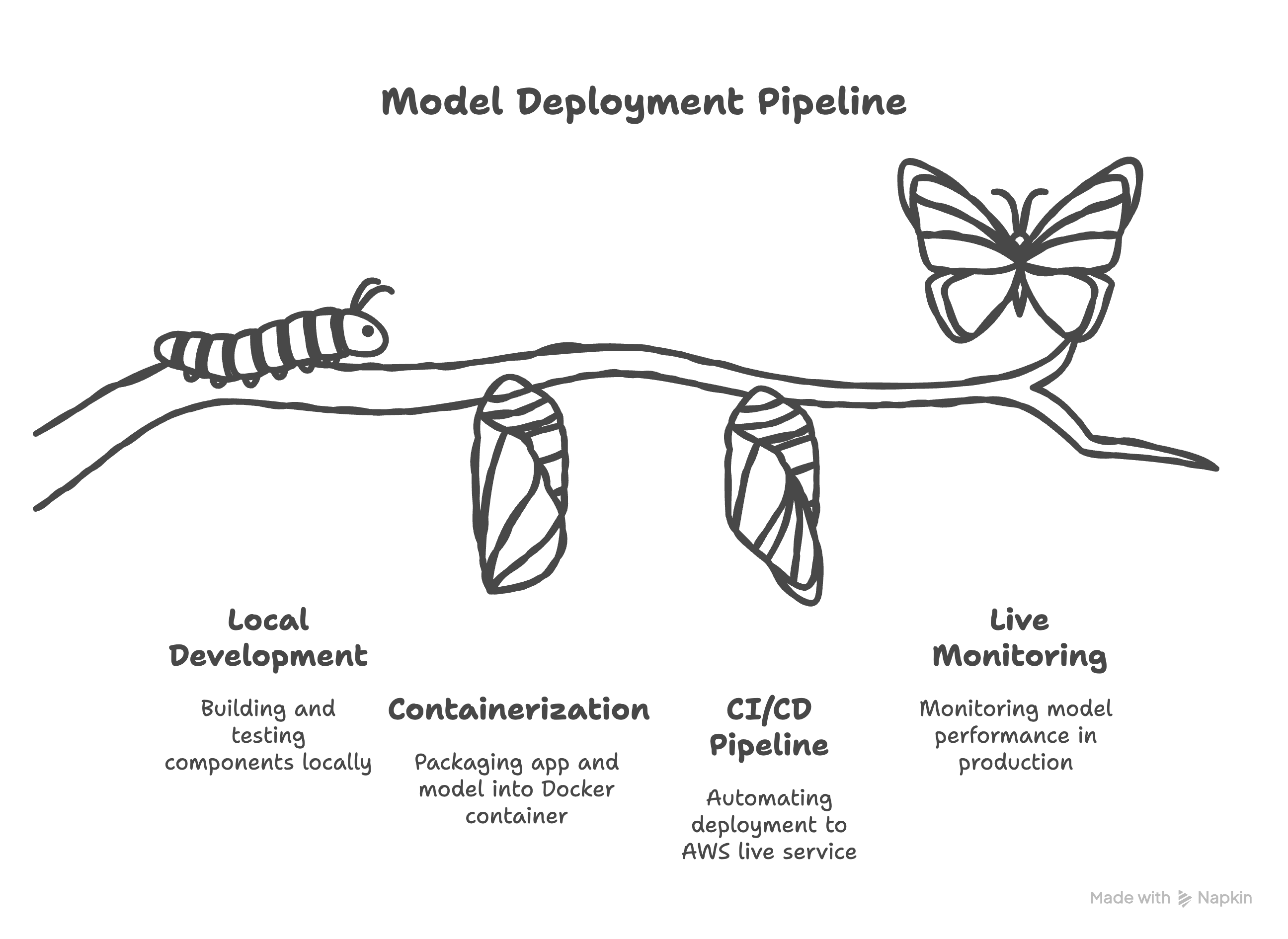
To make this journey digestible, we’ll break it down into four distinct acts. Each act represents a critical stage in taking a model from a local experiment to a production-grade feature.
Act I: The proving ground. We’ll build and test all our components locally, from setting up a professional repository and processing our data to systematically tracking our model experiments to find a winner.
The PM’s role here is to define success by choosing the right business metric (like the F1-score) and ensuring the team’s Definition of Done includes a full, auditable experiment log from a tool like MLflow.
Act II: The shipping container. We’ll use Docker to package the application and model into a standardized, portable container that can run reliably anywhere.
The PM’s role is to de-risk the deliverable by treating this container (and its
Dockerfileblueprint) as a non-negotiable acceptance criterion. This ensures the asset we’re building is portable and truly production-ready.
Act III: The assembly line. We’ll build the automated CI/CD pipeline that takes our container and deploys it to a live service on AWS with a single command.
The PM’s role is to enable velocity and reliability, framing the investment in this pipeline as a core product decision that directly improves release cadence and reduces deployment risk.
Act IV: The watchtower. Finally, we’ll discuss how to monitor the model in the wild to ensure it performs as expected and to catch any issues before they impact users.
The PM’s role is to protect the business value of the feature post-launch. We’ll frame monitoring as the insurance policy that prevents silent failure and protects our initial investment from degrading over time.
Project Resources: You can find the complete source code on GitHub and view the project presentation.
Ready to start building that bridge?
Your MLOps-to-English dictionary
Before we dive into the specific project, let’s start with the big picture: What is MLOps, really? At its core, it’s the set of practices for reliably and efficiently getting machine learning models into production. But for a PM, a better analogy is the factory assembly line.
Think of a data scientist’s model in a notebook as a brilliant, handcrafted prototype of a revolutionary engine. It’s a work of genius, but a prototype in a lab provides zero business value. MLOps is the entire factory you build around that engine. It’s the system that turns the bespoke prototype into a reliable, mass-produced feature that can be shipped globally, monitored for defects, and updated safely. Without the factory, the engine is just a cool experiment. With the factory, it’s a business asset.
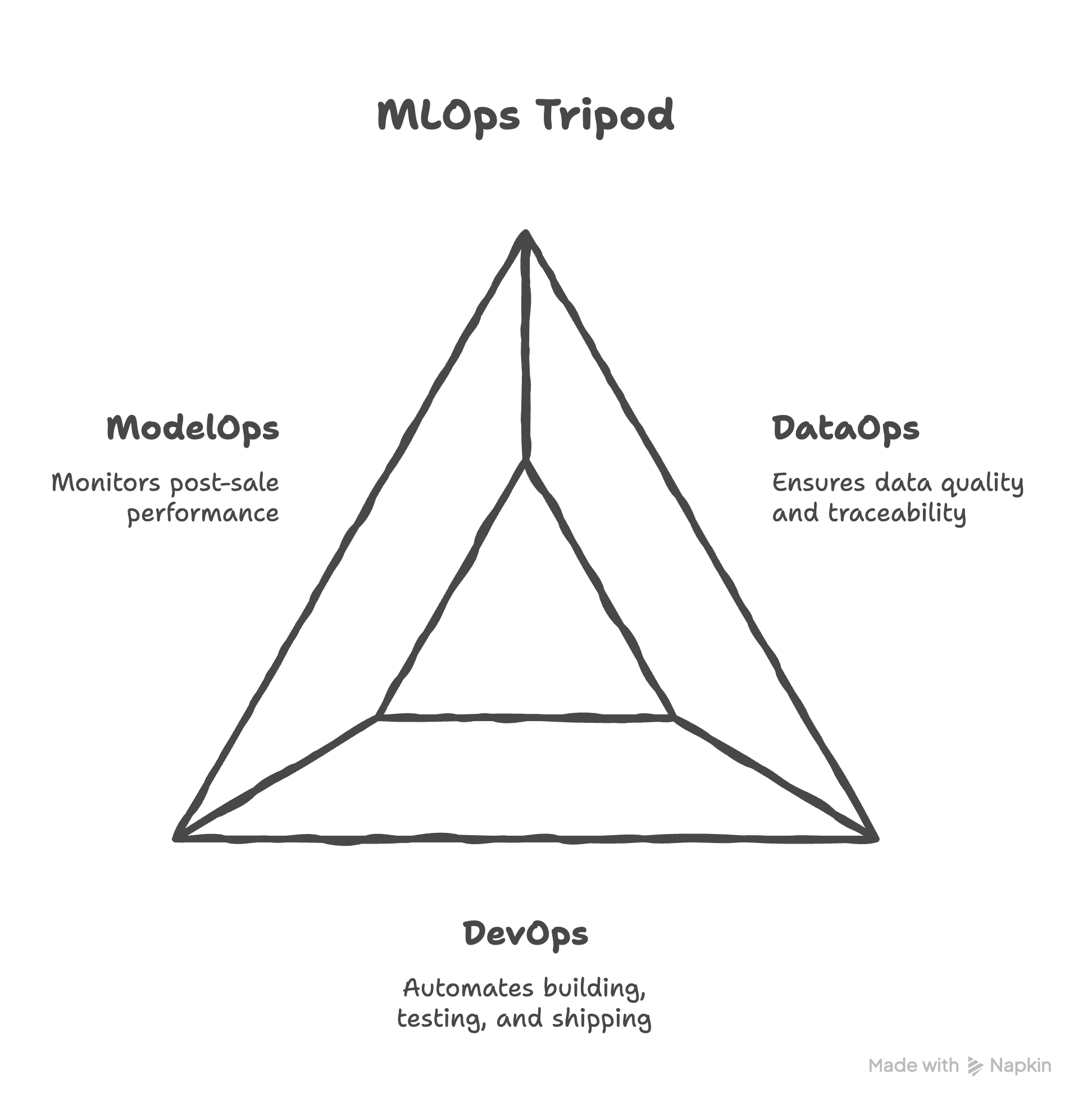
This factory has three main departments that you need to oversee. Think of it as the “tripod” of MLOps; if any leg is wobbly, the entire structure collapses.
DataOps, the raw materials warehouse: Manages the quality, consistency, and traceability of your most critical input, data.
DevOps, the assembly line machinery: The automation that builds, tests, and ships the product.
ModelOps, the post-sale support and recall team: Handles everything after the product has shipped, monitoring real-world performance.
Viewing MLOps this way reframes it from a technical practice into a business risk management framework, and that is squarely in the PM’s domain.
Git and GitHub: The project’s official history book
First up is Git. Created by Linus Torvalds in 2005 to manage the development of the Linux kernel, it’s the undisputed open-source standard for version control. For a PM, it’s the ultimate accountability tool. A good analogy is a shared Dropbox or Google Drive folder for a project. Think of Git as the local Dropbox folder on each team member’s computer. They can work on files, save versions (called “commits”), and have a complete history, even when they’re offline.
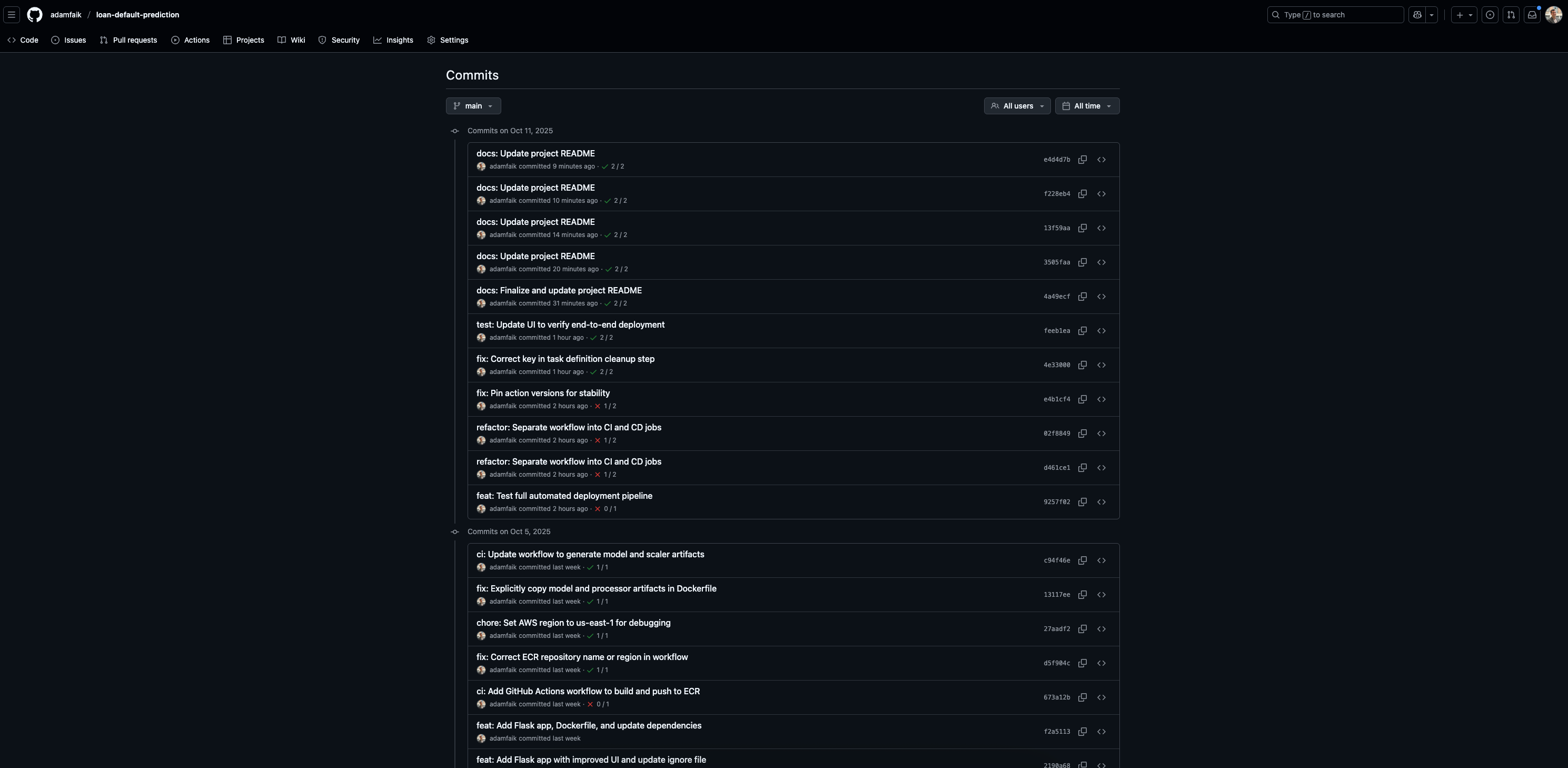
Then, GitHub (or alternatives like GitLab) is the central, shared folder in the cloud. When a developer is ready, they “push” their local changes up to GitHub, syncing the central folder for everyone else. As a PM, you care because this system creates a single source of truth. If a feature breaks, you can look at the history on GitHub and trace the problem back to the exact change that introduced it, providing a clear, non-negotiable audit trail.
MLflow: The scientific lab notebook
Data science is inherently experimental. To solve the “mess of models” problem, Databricks created and open-sourced MLflow in 2018. Think of it as the official, peer-reviewed lab notebook. While powerful alternatives like Weights & Biases exist, MLflow provides a clean way to systematically log every experiment. As a PM, this is crucial because it turns model selection from an art into a science. You can open the MLflow dashboard, sort all the experimental “runs” by the business metric you care about (like our F1-Score), and objectively see which version is the proven winner.
Docker: The sealed shipping container
You’ve probably heard the classic developer excuse: “Well, it works on my machine!” This problem is solved by containerization, a concept made accessible to everyone when Docker was released as open-source in 2013. It allows you to package your entire application, the code, the model, all specific library versions, into a sealed, standardized shipping container. It doesn’t matter where you run it; the contents inside work exactly the same. As a PM, you care because it massively de-risks deployment by eliminating an entire category of “it broke in production” issues.
CI/CD: The automated assembly line
Manually testing and deploying code is slow and error-prone. A CI/CD pipeline automates this. Modern tools like the open-source classic Jenkins, or integrated solutions like GitHub Actions (launched in 2018), make it easy to implement. Think of CI (Continuous Integration) as the Quality Control station: every time a developer submits a code change, a robot automatically runs tests. If they pass, CD (Continuous Deployment) acts as the Shipping Department, automatically packaging the app (using Docker!) and sending it to production. As a PM, you care because this means speed and reliability, allowing you to release improvements much faster.
Cloud services: The warehouse and factory floor
Once your “shipping container” is ready, you need a place to store it and a factory to run it. This is where cloud providers like Amazon Web Services (AWS), the market leader since 2006, come in. While alternatives exist on Google Cloud and Microsoft Azure, the concepts are similar. Amazon ECR is your secure, private Warehouse where your Docker containers are stored. Amazon ECS is the Factory Manager that takes containers from the warehouse and puts them to work, ensuring the right number are running and replacing any that break. As a PM, you care because these services ensure your application can handle real-world traffic and automatically recover from crashes, directly impacting user experience, uptime, and your budget.
Monitoring and observability: The post-sale support team
Finally, the MLOps lifecycle doesn’t end at deployment. A model’s performance is guaranteed to degrade over time as the real world changes, a problem called model drift. This is where monitoring comes in, acting as your “post-sale support.” Open-source tools like Arize or cloud-native services like AWS SageMaker Model Monitor are designed for this. They track your model’s live predictions and alert you when performance drops or the input data starts to look different from the training data. As a PM, you care because monitoring is your insurance policy against silent failure. It allows you to proactively schedule a “recall” (i.e., a model retrain) before a degrading model starts making bad decisions that cost the business real money.
Connecting the dots: The full MLOps story
Okay, that was a lot of definitions. It can feel like a list of disconnected tools. We’ll use them in the actual project in the next sections, but before we do, let’s connect all the pieces of the puzzle. Here is the complete story of how a model goes from a messy experiment to a reliable feature in your users’ hands.
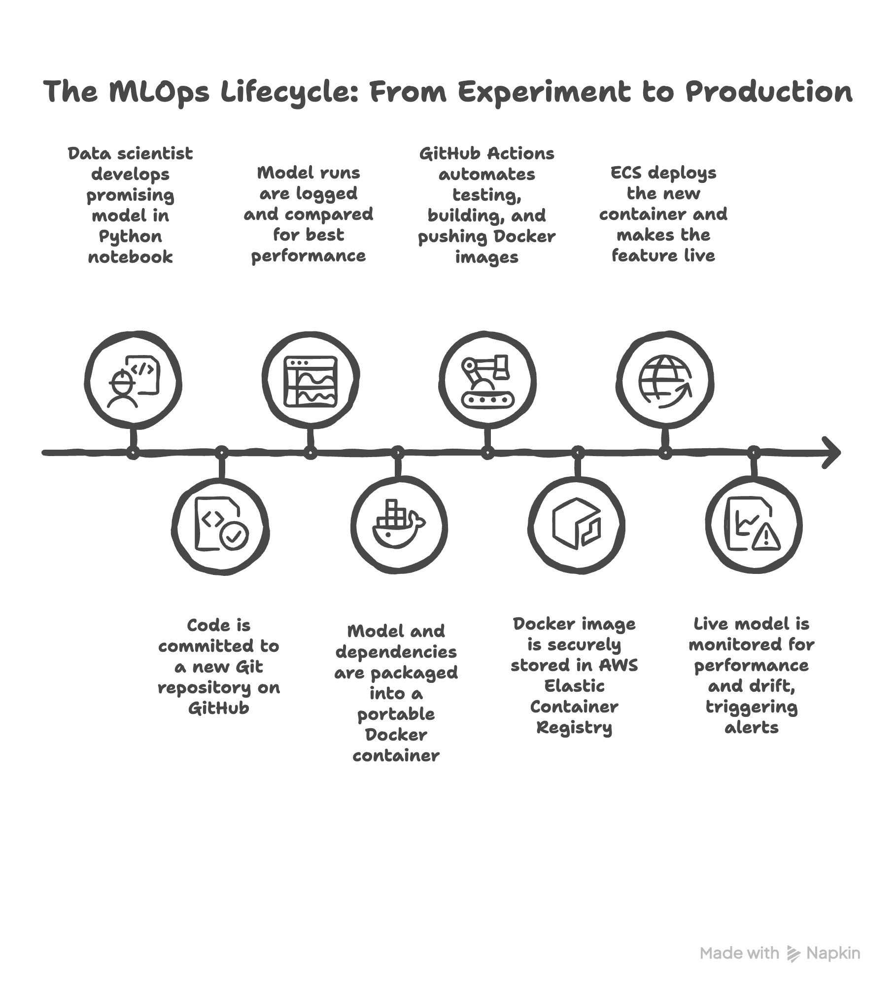
It all starts in the lab. A data scientist has a breakthrough in a Python notebook. They’ve built a model that shows incredible promise. The first step to professionalize this is getting the code into Git and GitHub. They initialize a repository, making that brilliant code the first entry in the project’s official history book.
As they experiment to improve the model, they don’t just save over their files. They use MLflow, the scientific lab notebook, to log every single run. Now, instead of a mess of files, you, the PM, can look at a clean dashboard and help them select the winning model based on the business metrics you defined.
Now we have a winning model file and the code that created it. To get it out of the lab, the team builds a simple web application around it. But to avoid the “it works on my machine” trap, they use Docker to package everything, the app, the model, the specific library versions, into a sealed shipping container. This container is now a portable, reliable, and versioned asset.
This is where the factory floor kicks in. Manually building and deploying this container is slow and risky, so we build our automated assembly line using CI/CD with GitHub Actions. A developer pushes a small code change to GitHub. This automatically triggers the Quality Control station (CI), which runs tests. Then, the Shipping Department (CD) takes over. It builds a fresh Docker container from the code, securely logs into our cloud “warehouse” (AWS ECR), and pushes the new container there.
The final step of the pipeline is telling the “factory manager” (AWS ECS) to deploy this new container. ECS takes the container from the warehouse, puts it on the factory floor, makes sure it’s running correctly, and makes it available to your users via a public URL. The feature is now live, and this entire process happens automatically in minutes.
But the story isn’t over. The factory’s “post-sale support team” takes over. Using a monitoring tool like Arize, we watch the live model for any signs of trouble. Is its performance degrading? Is it seeing strange new data? If the monitor detects a problem, like model drift, it sends an alert. This alert signals that it’s time to go back to the lab, retrain the model on new data, and the whole automated cycle begins again, ensuring the feature is not just deployed, but is continuously reliable.
Making the business case for MLOps
As a PM, your first job is often to justify the investment in building that factory. A data scientist might be excited about the model, but you have to convince leadership to fund the pipeline. MLOps isn’t just a technical practice; it’s a business risk management framework that delivers tangible, bottom-line benefits. Here’s how you can frame the ROI by contrasting the old way (a one-off model) with the new way (an MLOps pipeline).
First, consider the speed of innovation. Without a pipeline, updating a model is a manual, time-consuming process that can take weeks or even months of data science and engineering effort. With an automated MLOps pipeline, that entire process is reduced to hours or days. This faster time-to-deployment means you can update your fraud model monthly instead of quarterly, reacting to market changes much more quickly.
Next is deployment risk. The “one-off model” approach is prone to manual errors and the classic “it works on my machine” problem, making every release a nerve-wracking, high-stakes event. The MLOps “factory” approach minimizes this risk. Automated tests catch bugs early, and containerization guarantees that the application runs identically everywhere, from the lab to production.
Then there’s governance and auditability. In a traditional setup, the project’s history lives in disparate notebooks and local files, making it nearly impossible to reproduce a specific past prediction for a regulator. An MLOps pipeline provides ironclad governance. Git creates a perfect audit trail for every code change, while MLflow tracks every experiment, ensuring you can prove exactly how and why a model made a decision at any point in time.
Finally, think about scalability and reliability. A model stuck in the “lab” is often tied to a single person’s environment and requires manual intervention to run or recover from crashes. The MLOps approach uses cloud services like AWS ECS to build a system that is both scalable and self-healing. It can handle real-world traffic and automatically replaces any crashed containers, ensuring the high availability your users and the business depend on.
With this framework in mind, let’s dive into the use case that will guide us through the rest of this playbook.
The playbook in action: A 4-act journey
Enough theory. To really understand how the factory works, we need to build one. This next part of the article is the case study: a real-world project that will serve as our proving ground for every MLOps concept we’ve discussed.
The mission: The MLOps case study
Imagine you’re the product manager for a retail bank’s risk team. The business is in a tough spot. They’re facing unexpectedly high default rates on personal loans, which poses a significant financial risk to the institution. Your mission is to build a robust, automated system to predict the probability of a customer defaulting. The goal isn’t just to hand over a one-off model, but to create a reliable, end-to-end MLOps pipeline that can be trusted and updated over time.
Now, before we go any further, a crucial point: for this project, the specific machine learning model we choose doesn’t really matter. The dataset we’ll use is synthetic. The hero of this story is not a clever algorithm; it’s the MLOps pipeline we build around it. Our focus is 100% on the process, the reliable, repeatable system that can take any model from the lab to production.
Step one for the PM: defining what “good” looks like
Before a data scientist writes a single line of code, the PM’s first and most critical job is to define what success actually looks like. We have to translate the business problem into a clear, measurable technical target.
The project starts with a common and tricky data problem: imbalance. In the dataset, only 18.5% of the loans actually defaulted. (You can see the full Exploratory Data Analysis in the project notebook here).
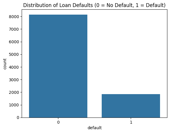
This imbalance makes the most common metric, Accuracy, a trap. For example, say 95% of customers don’t default and 5% do. A lazy model could just predict “No Default” for everyone and boast 95% accuracy! But it would be completely useless, because it missed every single default, potentially leading to catastrophic losses for the bank.
This forces us to look at a more nuanced trade-off, and this is a conversation every PM on an AI project should lead.
What is a “false positive”? This is when our model wrongly flags a good customer as a potential defaulter. The business impact? We might deny them a loan they would have paid back. We lose out on some business, but the damage is contained.
What is a “false negative”? This is when our model misses a customer who will actually default. The business impact? A direct financial loss for the bank, lost principal and interest. This is the catastrophic outcome we are trying to prevent.
For a bank, the cost of one big false negative is usually far, far higher than the cost of a few false positives. This business context dictates our strategy. We need a model that is excellent at finding as many of the real defaulters as possible, even if it means we sometimes flag a few good customers by mistake.
In machine learning terms, this means we must prioritize maximizing Recall (the ability to “recall” or find all the actual defaulters). To make sure the model doesn’t go too far and just flag everyone, we use a metric that creates a balance: the F1-Score. It’s a clever combination of Recall and its counterpart, Precision (how many of the flagged customers were actually bad). The F1-score becomes the single best metric to optimize for.
With the mission clear and our F1-Score chosen as the north-star metric, we’re ready to step into the lab and begin Act I of our journey: building and testing our components on the ground.
Of course. Let’s build out the first major section of our playbook. This is “Act I,” where we lay all the critical groundwork. I’ll maintain the conversational, PM-focused tone, integrating the practical steps from your project plan with the key learnings and narrative from your other documents.
Act I, the proving ground: From a blank folder to a winning model
This is where the real work begins. Act I covers everything we do locally, in the “lab,” before we even think about the cloud. This act is a blend of DataOps (establishing the repeatable data processing script) and ModelOps (running the systematic model bake-off). The goal here is to build a solid, professional foundation. It’s tempting to jump straight into a notebook and start building a model, but the MLOps way is to start with structure. This discipline is what separates a one-off experiment from a reproducible, production-ready asset.
The foundation: Professionalism from day one
Before writing any Python code, our first step was to treat this like a real software project. We started by creating a new repository on GitHub and cloning it to create a local folder. The very first thing we did was create a .gitignore file and make our initial commit.
This brings us to our first and most fundamental principle: Version control code, not artifacts.
A Git repository should be the “single source of truth” for the code and configuration needed to reproduce your results. It should not be a storage bucket for the files your code generates. These generated files are called artifacts. In the .gitignore file, we explicitly told Git to ignore things like:
Processed data files (e.g.,
data/processed/)The final model files (e.g.,
model.pkl)The MLflow experiment logs (
mlruns/)
As a PM, this is a critical concept. It ensures the repository stays lean and that the only way to get a model is by running the version-controlled code, which guarantees traceability. This discipline creates a transparent and auditable record of development from the very beginning.
The data pipeline: Guarding against data leakage
Like most data science projects, the initial exploration happened in a Jupyter Notebook. But for a production system, logic can’t live in a notebook. We immediately moved all our data cleaning and feature engineering steps into a repeatable Python script: src/data_processing.py.
This is where we encountered a classic and dangerous ML trap that every PM should know about: data leakage.
Data leakage happens when information from your test data accidentally “leaks” into your training process. The model learns an artificial shortcut that doesn’t exist in the real world, leading to “too good to be true” performance that will fail spectacularly in production.
To prevent this, we followed the golden rule: Split the data first. Any operation that learns from the data (like fitting a scaler to normalize values) must be done only on the training set. Those learned parameters are then applied to the test set. Enforcing this rule is a key part of the PM’s role in managing model risk.
The bake-off: Scientific model selection with MLflow
With a clean data pipeline, it was time to find our winning model. This is where we solved the “mess of models” problem. Instead of chaotic experimentation, we ran a systematic “bake-off” using MLflow.
We created a training script, src/train.py, and tested three different algorithms: Logistic Regression, Random Forest, and LightGBM. For each model type, we set up a distinct MLflow “Experiment”. Every time we trained a model with a different set of settings (hyperparameters), we logged it as a “Run”. We systematically recorded:
The input hyperparameters,
The resulting performance metrics (especially our north-star, the F1-Score),
The final model file itself as an artifact.
This turned model selection from a subjective guess into a data-driven decision. As the PM, I could open the MLflow dashboard, go to the comparison view, and simply sort all the runs by the F1-Score to scientifically identify the best-performing model.
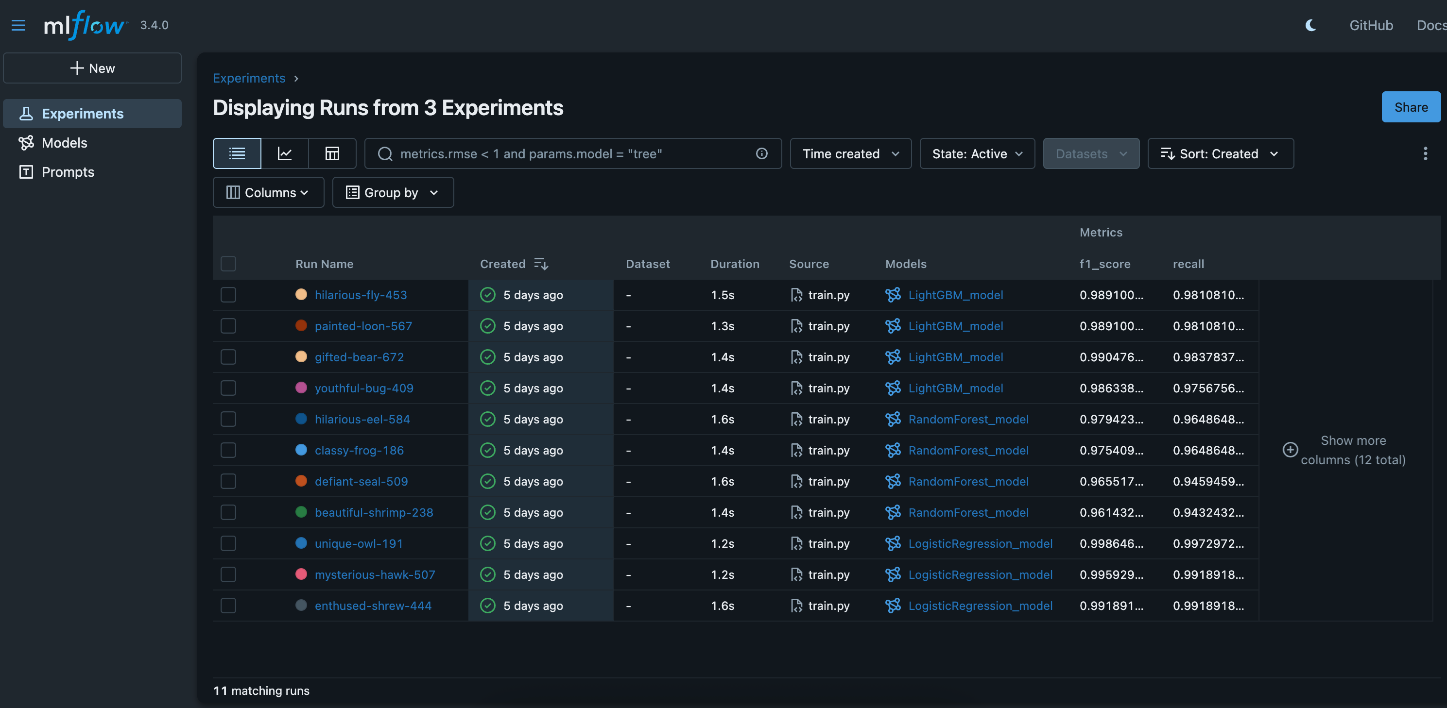
At the end of Act I, we have our champion: a Logistic Regression model that gave us the best balance of performance and simplicity. We have the clean, version-controlled code that can reproduce it, and a trustworthy evaluation to back it up. Now, we’re ready to package it for the factory.
Of course. We’ve got our winning model from the “Proving Ground” of Act I. Now, in Act II, we need to package it for the factory floor. This section details how we build our “shipping container.”
Act II, the shipping container: Packaging the model for production
At the end of Act I, we had a winning model file (model.pkl) and a data scaler (scaler.joblib) sitting on our local machine. But an artifact on a single computer is fragile and useless for a real product. To get it ready for the factory, we need to solve one of the oldest and most frustrating problems in software development: the “it works on my machine” headache.
A model that works perfectly for a data scientist might fail on a cloud server because of a different Python version, a conflicting library, or a missing dependency. This is where containerization becomes the PM’s best friend for de-risking deployment.
The solution is to package the entire application into a standardized, sealed shipping container using Docker. It doesn’t matter what server (the ship) it runs on; the contents inside are protected, isolated, and work exactly as intended every single time. This is a core DevOps practice that ensures the asset is standardized and portable.
Building the application and its blueprint
Our first step was to build a simple web application using Flask, a popular Python framework. This app.py script loads our model and scaler, presents a web form to the user, and returns a prediction.
With the app built, we created the blueprint for its environment: the Dockerfile. This is a simple text file that acts as a step-by-step recipe for building our container. Here’s the exact Dockerfile from the project, broken down line-by-line:
# 1. Start from an official, lightweight Python base image
FROM python:3.9-slim

# 2. Set the working directory inside the container
WORKDIR /app

# 3. Copy all project files into the container’s /app directory
COPY . .

# 4. Install all the Python dependencies listed in the requirements file
RUN pip install -r requirements.txt

# 5. The command to run when the container starts
CMD [”python”, “app.py”]
As you can see, the recipe is straightforward. It starts from a clean Python environment, copies the application code and model files inside, installs the necessary libraries from our requirements.txt file, and finally, tells the container how to start the Flask web server.
Testing the container locally
With the blueprint written, the final step was to build and test our container right on our local machine. We ran two simple commands:
docker build -t loan-default-app .This command reads theDockerfilerecipe and builds the final, portable package, which is called an Image.docker run -p 5000:5001 loan-default-appThis command takes the image and brings it to life as a running Container.
The moment you open your web browser to http://localhost:5000 and see your application running perfectly inside this isolated environment is a true “aha!” moment. We now have a self-contained, reliable, and version-controlled asset. Our model is no longer just a file; it’s a portable product, sealed in its container and ready for the automated assembly line of Act III.
Of course. Now we get to the heart of the MLOps factory. We have our perfectly packaged container from Act II. In Act III, we build the automated assembly line that takes this container and gets it to our customers without any manual intervention. This is where we connect all the pieces to achieve true, hands-free deployment.
Act III, the assembly line: Full automation with CI/CD
With the application sealed in a Docker container, we’ve solved the problem of consistency. Now we need to solve the problem of speed and reliability. Manually building an image, pushing it to the cloud, and deploying it is slow, repetitive, and a recipe for human error. The solution is to build an automated assembly line, a CI/CD pipeline. This is pure DevOps, building the automated machinery of the factory.
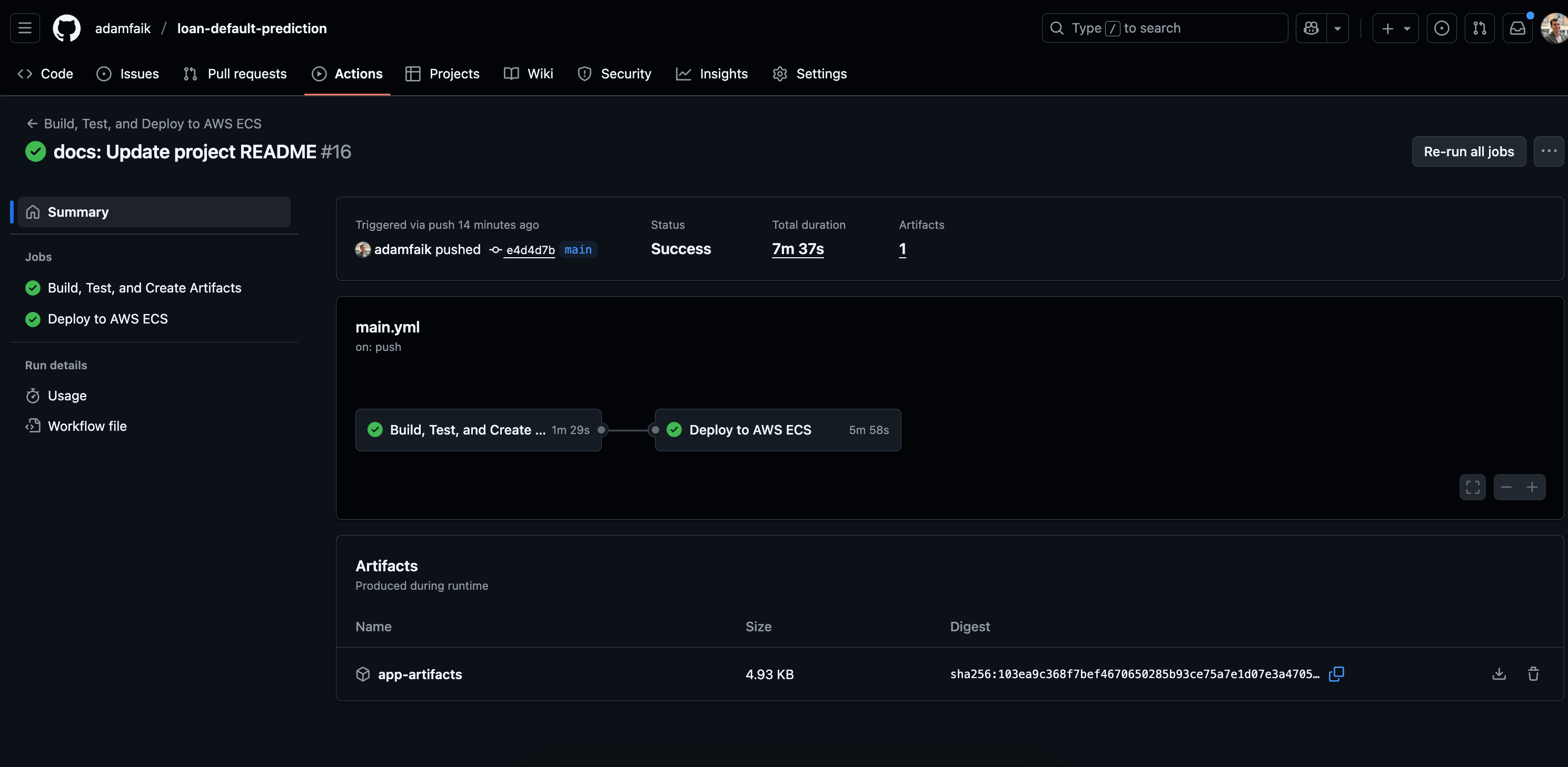
For this project, we used GitHub Actions, a powerful automation tool built right into GitHub. The entire logic for our pipeline is defined in a single text file: .github/workflows/main.yml. This pipeline automatically kicks off every time we push a change to our main code branch.
The “clean runner” problem: A critical MLOps lesson
When we first designed the pipeline, we hit a wall. The pipeline would fail because it couldn’t find the model.pkl or scaler.joblib files needed for the Docker build. This revealed a critical MLOps insight: your pipeline must be self-contained.
The GitHub Actions “runner” is a clean, empty virtual machine that starts from scratch on every run. Since we correctly ignored our artifacts in .gitignore, those files didn’t exist in the repository the runner cloned. The pipeline couldn’t just find the model; it had to create it.
This led us to design a robust, two-job pipeline, which is a best practice for MLOps.
Job 1, the quality gate: Continuous Integration (CI)
The first job, ci, acts as our automated quality control station. Its purpose is to verify our code and generate the artifacts needed for deployment. Here’s what it does:
Installs all the project dependencies.
Runs the data processing script (
src/data_processing.py) to create the scaler.Runs the training script (
src/train.py) to create the final model.Runs tests to validate the system. This isn’t just traditional code testing. For an ML system, this includes data validation (checking for schema changes or unexpected values) and model evaluation (ensuring the new model’s F1-score on a held-out test set meets our minimum business threshold).
Finally, if all tests pass, it bundles all the necessary application files, the scripts, the HTML template, and the newly generated model and scaler, and uploads them as a shareable artifact.
If any of these steps fail, the entire pipeline stops. No bad code or broken process can move forward.
Job 2, the shipping department: Continuous Deployment (CD)
The second job, cd, only runs if the ci job succeeds. This is our automated shipping department, responsible for getting our container to the cloud. Here’s its workflow:
First, it downloads the artifacts that the
cijob created.It securely logs into the private cloud warehouse, Amazon ECR (Elastic Container Registry). We chose ECR over a public registry like Docker Hub for its better security and seamless integration with AWS.
It then builds the Docker image using the
Dockerfile.It pushes the new, versioned image to the ECR repository.
Finally, it tells the factory manager, Amazon ECS (Elastic Container Service), to deploy this new image, updating our live application.
As a PM, it’s crucial to ensure this process is secure. We never write passwords directly in the code. All our credentials, like the AWS_SECRET_ACCESS_KEY, were stored safely in GitHub Secrets, an encrypted vault within the repository settings.
The result? A single git push command on a developer’s machine now triggers a fully automated, secure, and reliable deployment process that ends with an updated feature in the hands of our users.
git push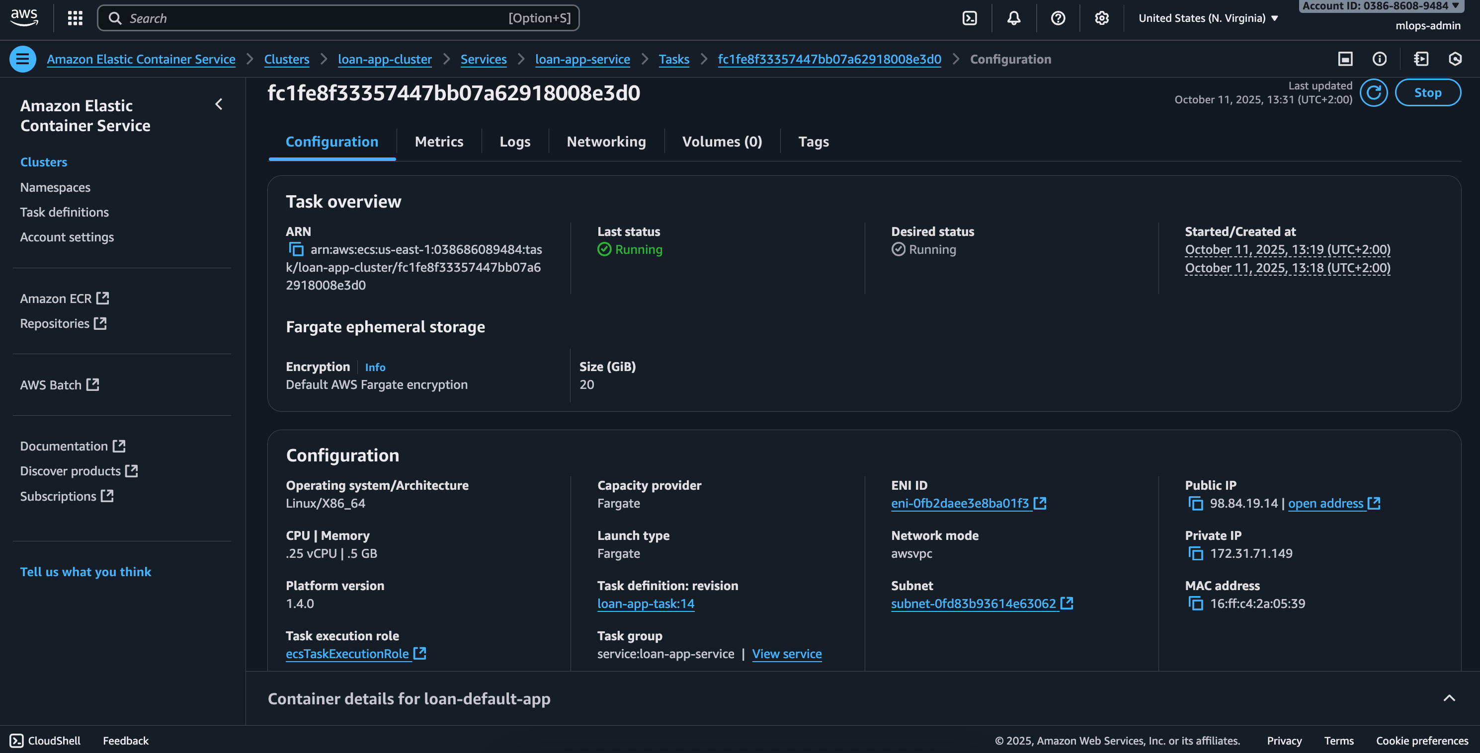
The debrief: Lessons from the factory floor
The assembly line is running, the feature is live, and predictions are being served. It’s tempting to mark the ticket “done” and move on to the next shiny object on the roadmap. But in MLOps, deployment is the starting line, not the finish line. The job is never truly done. This is where we shift from building the factory to operating it, and where the most critical long-term risks emerge.
Act IV, the watchtower: Monitoring for model drift
A model’s performance is not static; it’s guaranteed to degrade over time. It’s not a question of if, but when. This decay is caused by model drift, the primary threat to your model’s long-term value. As a PM, you need to budget for monitoring this from day one. Here, we return to the discipline of ModelOps, focusing on post-deployment performance.
There are two main types of drift you need to watch for:
Data drift: This happens when the live data coming into your model starts looking different from the data you trained on. Imagine a new marketing campaign suddenly brings in a flood of younger loan applicants. The input distribution has shifted, and your model, trained on an older population, may no longer be reliable.
Concept drift: This is trickier. It’s when the fundamental relationship between the inputs and the outcome changes in the real world. The classic example is an economic recession. Suddenly, having a high income might no longer be as strong a predictor of paying back a loan as it was before. The rules of the game have changed underneath your model.
To act as our “watchtower,” we integrated a monitoring tool like Arize into our application. The process is simple: with every prediction the live app makes, it sends the input features and the model’s output to the Arize dashboard. This allows us to track performance over time, get automatic alerts when drift is detected, and diagnose errors in specific segments of our user base.
However, this revealed a key PM constraint: ground truth delay. To calculate the live F1-score, we need to know if a customer actually defaulted. For a loan, that truth might not be known for months or even years. This means a PM must plan for a separate, often complex, data pipeline to eventually join the true outcomes back to the predictions, a significant project in itself.
Debugging in the trenches: What happens when the pipeline breaks
No MLOps journey is perfect. The deployment to the cloud involved solving several classic challenges. Here are the real-world errors I encountered and how I fixed them, the kind of issues your team will almost certainly face:
CannotPullContainerError: The ECS service couldn’t find the Docker image we pushed. The Fix: I had to ensure the Task Definition was using the full, specific image URI from ECR, including the unique tag (like the Git commit hash) that the pipeline generated for traceability.Container crashing (
Exit Code: 1): The application would start and then immediately crash. The Fix: This was a classic symptom of the “clean runner” problem. The CI pipeline wasn’t correctly generating and passing themodel.pklandscaler.joblibartifacts to the CD job, so the Docker container was being built without its most critical files.Connection refused: The container was running, but I couldn’t access the web app from the browser. The Fix: This was a networking issue. I had to correctly configure the AWS Security Group (the virtual firewall) to allow incoming traffic on the right port, and ensure the ECS Port Mapping correctly connected the public port to the internal port the Flask app was listening on.
As a PM, you don’t need to know how to fix these errors, but you should budget for them. Acknowledging that cloud deployment involves a “last-mile” of debugging for networking and permissions is key to setting realistic timelines.
A critical final step: Cleaning up to avoid costs
This might be the most important piece of practical advice for any PM overseeing cloud-based projects. Cloud services are pay-as-you-go. A resource left running, even if it’s idle, is still racking up a bill. I have seen small experimental projects accidentally generate five-figure AWS bills because someone forgot to decommission resources properly.
As the PM, you have to be the grown-up in the room and enforce a mandatory cleanup procedure. To avoid leaving orphaned, costly resources behind, you must tear down your AWS infrastructure in a specific order:
Stop the containers: First, update the ECS Service and set the “Number of tasks” to 0.
Delete the service: Once no tasks are running, you can delete the service itself.
De-register the blueprint: De-register all versions of the Task Definition.
Delete the cluster: Now that the cluster is empty, you can delete it.
Delete the artifacts: Finally, go to ECR and delete the repository that holds your Docker images.
Following this sequence ensures you stop the billing clock from ticking.
Your MLOps cheat sheet: Key learnings for PMs
We’ve been through the entire journey, from a blank folder to a live, monitored application. We’ve defined the jargon, walked through the four acts of the project, and debugged the issues along the way. Now, let’s distill all of that into five actionable principles that you, as a product manager, can bring to your next AI project.
Think in pipelines, not models
The biggest mental shift in MLOps is realizing that the machine learning model is not the most valuable asset you’re building. The model is a temporary artifact; it will degrade and need to be replaced. Your most valuable asset is the automated, repeatable, and reliable pipeline that produces the model. This factory assembly line is what gives your product speed, reliability, and the ability to adapt. When you advocate for MLOps, you’re not just investing in a single model; you’re investing in the machinery that will deliver value for years to come.
Containerization is non-negotiable
The “it works on my machine” problem is one of the biggest sources of risk and delay when moving from the lab to production. Containerization with a tool like Docker is the solution. By packaging your application, model, and all its dependencies into a sealed, portable container, you guarantee that it will run identically everywhere. As a PM, you should consider a Dockerfile a required deliverable from day one to de-risk every future deployment.
Instrument everything
You wouldn’t ship a product without analytics; don’t ship a model without instrumentation. This happens at two key stages. First, in the lab, use a tool like MLflow to systematically track every experiment. This turns model selection from a subjective guess into a scientific, data-driven decision based on the business metrics you care about. Second, in production, use a monitoring tool to track live predictions. This is your insurance policy against silent failure, allowing you to catch model drift before it starts making bad decisions that cost the business real money.
Secure by design
An automated pipeline that has the power to deploy to production needs to be incredibly secure. Never allow secret keys or passwords to be written directly into code or configuration files. Enforce the use of dedicated, least-privilege IAM Users for programmatic access to the cloud. All sensitive credentials, like your AWS keys or database passwords, must be stored in a secure vault like GitHub Secrets and accessed by the pipeline at runtime.
Deployment is the starting line, not the finish line
Finally, remember that the MLOps lifecycle is a continuous loop, not a linear path. The moment a model is deployed is the moment it starts to potentially degrade. As a PM, you must budget time and resources for this reality. This means planning for post-deployment monitoring, creating a process for periodically retraining the model on fresh data, and using the insights from your monitoring tools to guide the next iteration of the product. The project is never truly “finished.”
Your turn to build the bridge
We started this journey with a common problem: the intimidating gap between a promising machine learning experiment and a reliable, production-ready feature. My goal was to turn that technical black box into a transparent assembly line that any product manager could confidently oversee.
By walking through this project, from a blank folder to a fully automated pipeline, we’ve seen how MLOps isn’t just a set of tools, but a framework for managing risk and delivering value. The journey from feeling like I was managing a black box to understanding the factory floor has been transformative. My hope is that this playbook has demystified the process for you, too.
Now you have the vocabulary and the roadmap. You understand the “why” behind the “how.” The next time a data scientist shows you their brilliant model in a notebook, you’ll know exactly what questions to ask and how to start building the bridge to production. Your journey into leading AI products with confidence starts now.
What’s your experience been with the gap between the lab and the factory? Have you experimented with automating parts of your ML workflow, or are you just finding your starting point?
Thanks for this E2E deep-dive, Adam. I have a couple of questions about the MLOps work you did, if you don't mind me asking,
- What was the course you referred to from a Professor in your article?
- How long did this project take you?
- Did you learn AWS, Docker and SageMaker, or was that with help from someone else?
- Were you using Anaconda Jupyter Notebooks with MLFlow on your laptop initially?
- How did you build the presentation in GitHub?
I appreciate you sharing your process and tools you used.