
How to build a deep learning image classifier
My journey building an image classifier from 83% to 92% accuracy, sharing the code, concepts, and hard-won lessons that demystify the black box.

Many thanks to my deep learning professor at Sorbonne University, Dafnis Krasniqi, for his excellent course and for suggesting this very project.
If you’re a product manager in tech today, you’ve probably been in a meeting where the conversation turned to AI and suddenly felt like the engineers were speaking a different language. Terms like “neural networks,” “training epochs,” and “loss functions” get thrown around, and you’re left nodding along, trying to connect the technical jargon to the user problem you’re trying to solve. The core technology can feel like an intimidating black box.
I decided the best way to truly understand it was to dive in and write the code myself.
This article is the story of my side project: a journey to teach myself the fundamentals of deep learning by building an image classification model from the ground up. It’s written for product managers, by a product manager. My goal isn’t to turn you into a machine learning engineer, but to demystify the process through a real, practical example. We’ll follow a story in three acts: starting with a simple MVP model, making it smarter with modern techniques, and finally, leveraging the work of industry giants to achieve a world-class result, improving the model’s accuracy from a respectable 83% to a phenomenal 92.94%.
This is everything I wish I had known when I started, a practical guide to understanding not just how the technology works, but how to think about it from a product perspective. I’ve shared the complete, commented code in a Kaggle notebook (link here) for you to follow along or fork for your own projects.
Content
Deep learning 101: The PM’s technical briefing
Alright, before we dive into the project itself, let’s grab a virtual coffee and cover a few key ideas. When I started, terms like “convolution” and “softmax” felt like a completely different language. But once I got the hang of the core concepts, everything else clicked into place. Trust me, understanding these few building blocks will make the rest of the story, the failures, the breakthroughs, and the “aha!” moments, make so much more sense.
For a fantastic and more detailed explanation of all the theoretical concepts in this section, I highly recommend the lectures from Joaquin Vanschoren, which I used extensively throughout my learning journey (link here).
The basics: how a neural network “thinks”
First, let’s talk about a standard neural network. Forget images for a second; just think about a machine that learns from data.
The fundamental unit: a single neuron
The simplest way I found to think of a single neuron is as a tiny, simple decision-maker. At its core, it does something very similar to a basic linear regression model: it takes a set of inputs, multiplies each one by a “weight” to signify its importance, and adds them up. Then, to make a decision, it passes this result through an Activation Function (we’ll cover those in a bit) to produce a final output, like a “yes/no” or a score.

One neuron on its own is not very smart, but they are the fundamental building block.
Building the team: The network structure
But what happens when you get a whole team of these analysts and organize them into an org chart? Now you have a neural network, which is really just a succession of these simple models stacked in layers.
The input layer: This is the mailroom. It receives the raw data, the initial numbers, and passes it on.
The hidden layers: These are the specialized departments where the real work happens. The mailroom passes the data to the first department of analysts. They make their simple decisions and pass their outputs to the next department, which looks for more complex patterns in what the first group found.
The output layer: This is the CEO’s office. It takes the final, highly-processed information from the last hidden layer and makes the single, final decision, like “this is a cat” or “this product gets a 4-star rating.”

The more hidden layers and neurons you add, the more complex and subtle the patterns your network can learn. However, this complexity comes with a risk: a model that is too complex can overfit. This happens when the model learns the training data too well, including its noise and quirks, and as a result, it performs poorly on new, unseen data. You can spot overfitting on a chart when the training error continues to go down, but the error on your validation (or test) data starts to go up.
The school of AI: how a network learns
So how does this team of analysts go from making random guesses (initialization with random weights) to making smart predictions? They go through a training process, which is an iterative optimization loop of “guess, check, and correct.”
Think of it like teaching a student:
Forward pass: You show the student a picture (the input data) and they make a guess (”I think it’s a dog”).
Loss calculation: You compare their guess to the right answer (”It’s actually a cat”) and use a loss function to give them a score for how wrong they were. This “error score” is called the loss. A high loss means a very wrong guess.
Backward pass (Backpropagation): This is the magic step. An optimizer (like Gradient Descent) thinks backward about why the student was wrong. It calculates how much each internal weight contributed to the error.
Weight update: The student adjusts their thinking process for next time. The optimizer makes tiny adjustments to all its weights, nudged in the direction that will reduce the error.

This entire loop is one training step, or iteration. The model repeats this process for each small batch of images. Once it has seen all the images in the entire training dataset one time, we say it has completed one epoch. You then repeat this entire process for multiple epochs, and slowly but surely, the network’s guesses get better.
The training dials: key hyperparameters
When you set up this training loop, you have a few key “dials” or settings to control it. These are called hyperparameters.
Epochs: An epoch is one full pass through the entire training dataset. How many times should the student review the whole textbook? Too few, and they won’t learn enough. Too many, and they might start to memorize (overfit).
Batch size: Instead of showing the student every single photo before they update their thinking, we show them a small “batch” (e.g., 32 images) and then let them update their weights. This is much more computationally efficient.
Learning rate: This is probably the most important dial. It controls how big the weight adjustments are after each batch. A high learning rate means taking big steps, which can learn fast but might overshoot the best solution. A low learning rate means taking tiny, careful steps, which is more precise but can take a very long time. There’s an inverse relationship here: if you’re training for many epochs, you typically want a smaller learning rate to make careful refinements.
The “style” of a neuron: activation functions
Activation functions are crucial because they introduce non-linearity, allowing the network to learn relationships far more complex than a simple straight line. Think of it as giving each analyst a specific “communication style.”
ReLU: The most common style for hidden layers. It’s a “go/no-go” analyst. If the information is important (positive), they pass it on. If not (negative), they say nothing (output zero). It’s simple and very efficient.
Sigmoid and Tanh: These are older styles that compress the output. Sigmoid squishes it between 0 and 1, while Tanh squishes it between -1 and 1. You don’t see them as often in hidden layers anymore, but Sigmoid is still useful for binary (yes/no) output layers.
Softmax: The “committee chairperson” for the output layer in a multi-class problem like ours. It takes all the final scores for every category (forest, sea, etc.) and converts them into a set of probabilities that add up to 100%. The category with the highest probability is the winner.


A universal language: one-hot encoding
One last foundational piece. A neural network only understands numbers. It has no idea what “forest” or “sea” means. So how do we feed it the correct labels? We use one-hot encoding.
Imagine a set of light switches, one for each of our six categories. To represent the “forest” category, you simply flip the ‘forest’ switch ON (1) and make sure all the other switches are OFF (0). The label for “forest” becomes a vector like [0, 1, 0, 0, 0, 0]. This prevents the model from thinking there’s a weird order to the categories (e.g., that street (5) is greater than forest (1)). It’s a simple and essential way to prepare categorical data for a model.
The image specialists: convolutional neural networks
Okay, so that’s a standard network. It’s great for data in a spreadsheet, which is a 1D vector. But for images? We need a specialist: the Convolutional Neural Network (CNN), a type of deep learning model designed to automatically learn patterns from grid-like data.
How a computer really sees a picture: tensors
The first “aha moment” for me was realizing that a computer doesn’t see a photo as a single flat thing. It sees a tensor, which is the fundamental data structure in machine learning. Think of it as a multi-dimensional array. For a color image, it’s a 3D tensor: three distinct matrices (spreadsheets of numbers) stacked on top of each other, one for the Red pixel values, one for Green, and one for Blue (RGB). The entire job of a CNN is to intelligently process this tensor.
Inside the CNN assembly line
I think of a CNN as a feature-finding assembly line that deconstructs an image. A standard neural network would be overwhelmed by the tens of thousands of pixels in a high-resolution image. The CNN’s reduction process is essential.
Step 1: The feature detector (convolution layer). The core of a CNN is convolution. This is a mathematical operation where a small filter (or kernel), like a 3x3 pixel magnifying glass, slides over the input image. At each position, it creates a “feature map” that highlights specific features like edges, corners, or textures. The network has many of these filters, each learning to find a different pattern. (A quick technical note: this process sometimes involves zero padding, or adding a border of zeros around the image, to make sure the filter can process the edges properly).
The image below gives a fantastic visual for this. The top row shows what some of these specialized filters or “magnifying glasses” look like, some are designed to find vertical lines, others horizontal blurs, and some even find diagonal textures. The rows below show the result of applying each filter to an image of a boot or a shirt. Notice how each filter highlights a completely different aspect of the original image, creating a unique “feature map” that captures a specific piece of information.

Step 2: The summarizer (max-pooling layer). After finding all these detailed features, we need to summarize them. The most common way is max-pooling. It takes a small window (e.g., 2x2) of the feature map and keeps only the single biggest number. This might sound like it’s throwing away data, but this reduction in quality is actually a good thing! It makes the model faster, more efficient, and forces it to focus only on the most prominent features it found.

Step 3: The bridge (flatten layer). After several rounds of convolution and pooling, the network has built a rich but complex set of 2D feature maps. But the final decision-making part of our network, the standard “dense” layers, needs a simple, flat, 1D list of numbers. The Flatten layer is the crucial bridge that does this conversion, turning the multi-dimensional tensor into a long vector.
Step 4: The Decision-Maker (dense layers). Finally, this long vector is fed into a standard set of neural network layers (the “CEO’s office”) which makes the final classification.
Okay, that’s the playbook. Now that we speak the same language, let’s get into the real story.
The mission: from pixels to product intelligence
More than just pixels
Imagine you’re the PM for a new feature in a major travel app. The goal? Automatically categorize the millions of photos users upload: sun-drenched beaches, bustling city streets, serene mountain peaks. This isn’t just about creating tidy albums; it’s about powering personalized recommendations, enhancing search, and creating truly magical user experiences. But how do you teach a machine to see the difference between a glacier and a snow-capped mountain? That was the exact challenge I set for myself.
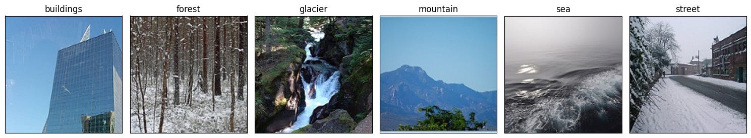
My mission was to transform raw pixels into intelligent scene understanding. I chose the Intel Image Classification dataset as my digital world to conquer. It’s a comprehensive collection of over 25,000 images spanning six distinct categories: buildings, forest, glacier, mountain, sea, and street. The real-world complexity of this dataset made it the perfect proving ground.
My journey unfolded in three distinct acts. First, I built a simple model from scratch to establish a baseline. Then, I made it smarter with modern techniques designed to improve learning. Finally, I achieved a massive breakthrough by, quite literally, standing on the shoulders of giants. Along the way, I hit surprising failures, critical ‘aha’ moments, and learned lessons that every product leader in the AI space needs to know.
The challenge: a mountain or a glacier?
The task was clear: build a model that could look at any of the 25,000+ images and accurately assign one of the six labels. Early on, as I explored the data, one problem became immediately obvious, and it would follow me through every experiment: the persistent confusion between “glacier” and “mountain” scenes.
To a human, the difference might seem clear: one is primarily ice, the other rock. But to a machine learning model, both are vast landscapes featuring white peaks, rugged terrain, and a lot of sky. This visual similarity became my benchmark, my narrative antagonist. Any model I built had to prove it was smart enough to solve this specific, tricky problem.
For a product manager, this is a critical lesson. My personal goal for this project was to push the limits and see if I could break the 90% accuracy barrier. But in a real-world product scenario, the first question is always: what is an acceptable mistake? If a travel app mislabels a glacier as a mountain, is that a critical failure? Probably not.
The key is to define the cost of being wrong for your specific use case. Success isn’t just about the highest possible accuracy score; it’s about finding the right trade-off. An 80% accurate model that can be developed quickly and with fewer resources might be a much better fit for the business, especially if we design the product to handle potential errors, for example, by adding a feature for users to correct a classification, creating a “human-in-the-loop” system. Your model’s ability to handle ambiguous cases is important, but your product’s ability to handle the model’s inevitable mistakes is where true value and user trust are won or lost.
On a positive note, my initial data exploration revealed that the classes were relatively balanced, with each category having a roughly similar number of images.
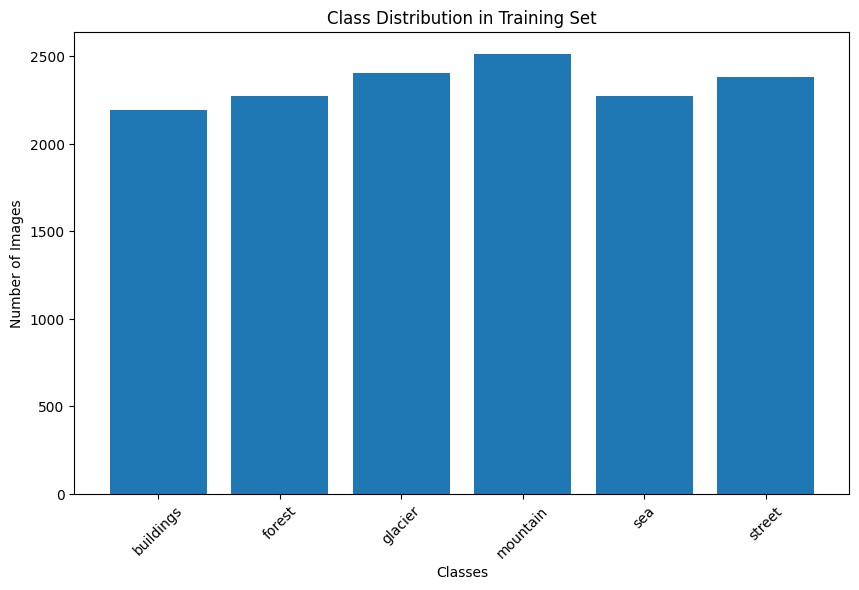
This was a small but significant piece of good news. In many real-world projects, you might have 10,000 photos of one class and only 100 of another. This forces you to use special techniques like undersampling (deleting samples from the majority class) to avoid the model becoming biased. I was lucky to not have to worry about that. With the challenge defined and my antagonist identified, I was ready to build my first contender.
The workshop: setting the stage for the experiments
With a clear mission, it was time to set up my workshop. For any product, the tools and preparation you do upfront can make all the difference between a smooth project and a frustrating one. This was no different.
Choosing the workshop: why Kaggle?
Every project needs a home. For this one, I chose Kaggle, a fantastic all-in-one platform for data science that provides a powerful, free online coding environment called Kaggle Notebooks. Think of it as a combination of a supercharged Google Docs for code, a massive library of datasets, and a community of experts.
From a PM perspective, the business case was a no-brainer. Training deep learning models takes a huge amount of computational power. Trying to do it on my laptop would be like trying to bake a cake in an easy-bake oven. Kaggle, on the other hand, gives you free access to powerful GPU accelerators for a generous number of hours each week. These are the industrial convection ovens of the AI world, and they were a game-changer, allowing me to run experiments in hours, not days.
The other killer feature is its integrated dataset library. This is where Kaggle really shines compared to similar tools like Google Colab. While both are great, Kaggle allows you to add massive datasets like the one I used to your project with a single click, no messy downloads or Google Drive connections required. It’s this kind of seamless workflow that makes it perfect for rapid experimentation.
One quick practical tip: If you need to install any external libraries, you have to enable internet access in the notebook’s settings. It’s a simple toggle in the “Session options,” but it’s a crucial step that might require a one-time phone number verification. It’s a small hurdle to clear for all the power you get in return.
Building a reusable toolkit: helper functions
Before diving into the experiments, I took a step that every good engineer and product manager should appreciate: I built a set of reusable tools. In coding, these are called helper functions. Instead of writing the same block of code over and over again to visualize results, I wrote a function once and then simply called it whenever I needed it. This not only saved a ton of time but also ensured that every model was evaluated in exactly the same way, making the comparisons fair and consistent.
For this project, I created four key helpers:
plot_history: To visualize the training and validation accuracy/loss curves.evaluate_model: To generate a detailed classification report and confusion matrix.visualize_predictions: To see how the model performed on a random batch of images.visualize_grad_cam_analysis: The “highlighter” tool to peek inside the black box (more on that later).
The golden rule: train/validation/test split
This is perhaps the most important concept in all of machine learning. You can have the best model in the world, but if you don’t evaluate it correctly, your results will be meaningless. The golden rule is to split your data into three separate buckets before you do anything else.
Think of it like studying for a big exam:
Training set (80% of our data): These are the practice questions and textbook chapters you study from. The model sees these images and their labels to learn the patterns.
Validation set (20% of our data): This is the mock exam you take a week before the final. You use it to check your progress, see where you’re weak, and tune your study strategy (i.e., tune your model’s hyperparameters). The model doesn’t learn from this data, but we use its performance on this set to make decisions.
Test set (a completely separate folder of data): This is the final exam. The model has never seen this data before. You only use it once, at the very end, to get a final, unbiased score of how well your model will perform in the real world.
Following this process prevents a critical error called data leakage. This happens if information from your validation or test sets accidentally “leaks” into your training process. If you normalize your data or select features before splitting, the model has already learned something about the entire dataset, and its final score will be artificially inflated. You have to pretend the test set doesn’t even exist until the final evaluation.
In the project, Keras’s ImageDataGenerator made this easy by allowing me to specify a validation_split to automatically create the training and validation sets. The test data was already in a separate folder (seg_test) to ensure it remained untouched until the very end.
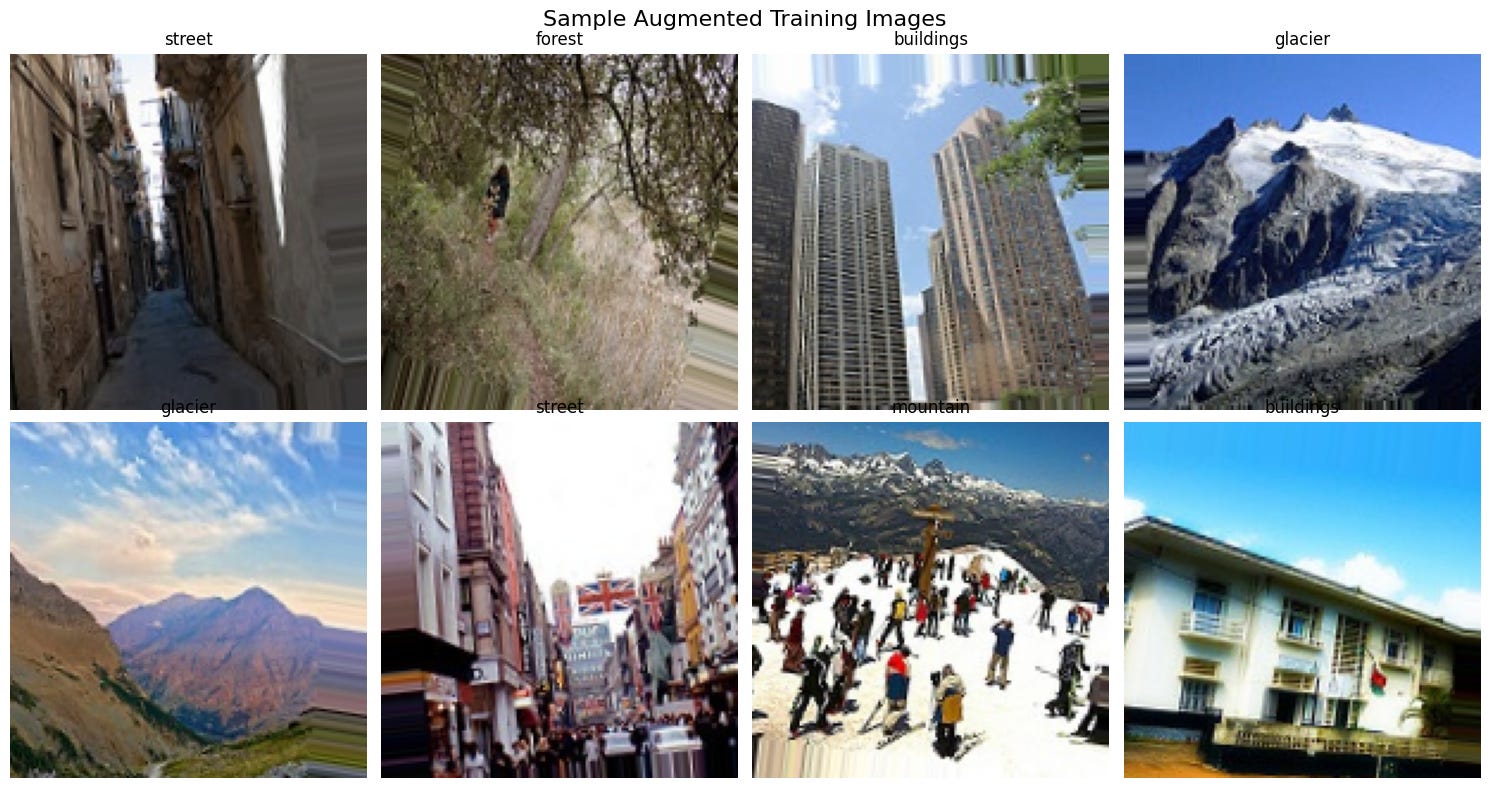
The smart copy machine: data augmentation
With my data safely split, it was time to apply the data augmentation strategy to the training set only. It’s a technique to artificially increase the size of the training set by applying various transformations to the existing images.
The analogy is simple: it’s like taking a single photo of a street and creating a whole album from it. You flip it horizontally, zoom in a little, rotate it slightly, and maybe shift it a bit. To a computer, each of these small transformations creates a brand new, unique image. This process teaches the model a crucial concept called invariance, that a ‘street’ is still a street, even if viewed from a different angle. It’s one of the most effective and cheapest ways to help a model generalize and avoid overfitting.
With my workshop set up, my tools built, and my data strategy in place, I was finally ready to start the main event.
The journey in three acts
This is where the real action happens. My journey from a simple proof-of-concept to a world-class classifier unfolded in three distinct acts.
Act I: The baseline MVP (83% accuracy)
Every AI project needs a starting point, a baseline. Mine was a simple CNN built from scratch. Think of it as the Minimum Viable Product. The goal wasn’t perfection; it was to prove the concept was viable and to get a score on the board that we could improve upon.
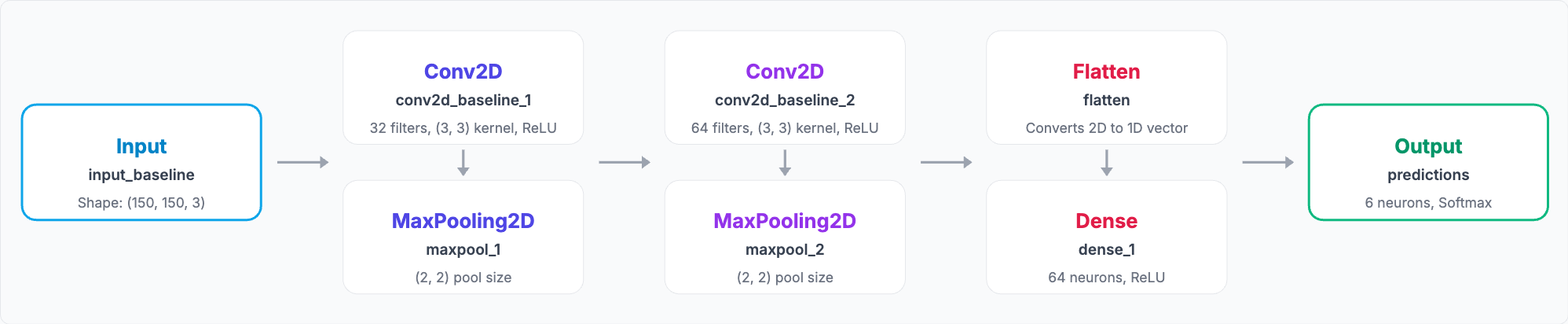
Here’s the blueprint for that first model. It was a straightforward implementation of the CNN assembly line, built with two main blocks.
The first block was designed to find simple, fundamental features. A Conv2D layer with 32 filters would scan the image for basic patterns like edges, corners, and color gradients. Immediately after, a MaxPooling2D layer would act as a summarizer, shrinking the resulting feature maps and keeping only the most important information.
The second block then took these summarized features and looked for more complex patterns. Another Conv2D layer, this time with 64 filters, combined the simple edges and corners into more meaningful shapes. This was followed by another MaxPooling2D layer to further condense the information.
Finally, this highly processed data was fed into the “CEO’s office,” a classification head. A Flatten layer converted the 2D feature maps into a long 1D list, which was then passed through a final Dense layer to make the ultimate prediction for our six categories.
I trained the model for a maximum of 20 epochs, but used an early stopping callback. This is a simple but powerful technique that monitors the validation loss and stops the training automatically when it stops improving, which prevents overfitting and saves a lot of time.
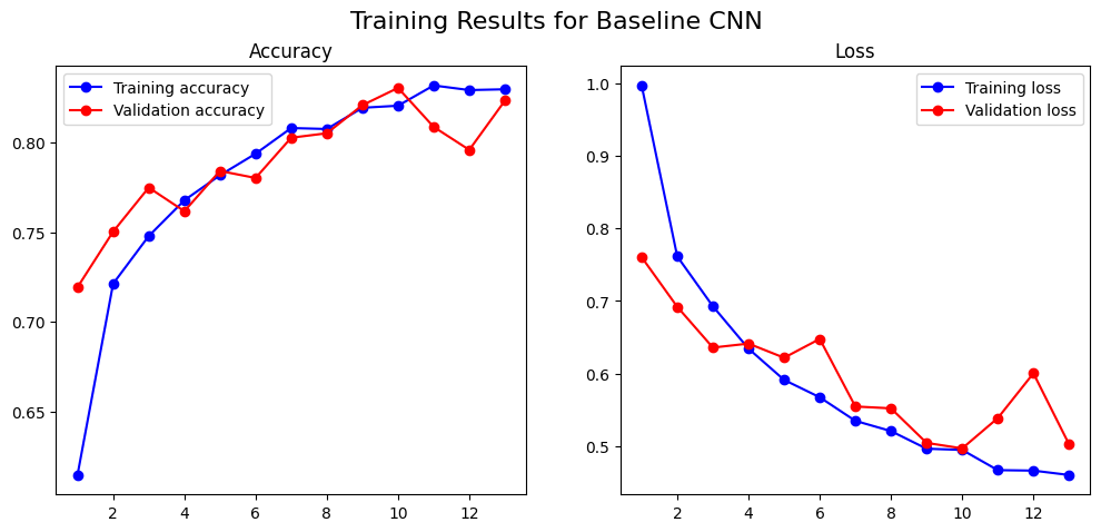
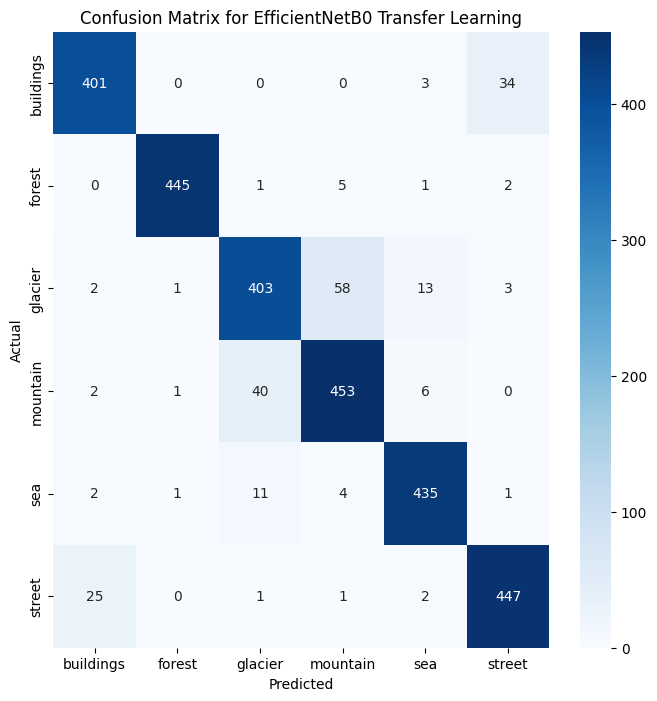
The result was 83% accuracy. A huge win. But an overall accuracy score is like a company’s revenue number: it tells you if you’re winning, but not where. For that, we needed the confusion matrix. This is a product manager’s best friend for diagnosing a classifier. It’s a simple table that shows you exactly what the model predicted versus the actual truth. The diagonal line from top-left to bottom-right is the good news: it shows all the correct predictions. Everything off the diagonal shows an error, revealing precisely where the model is getting “confused.”
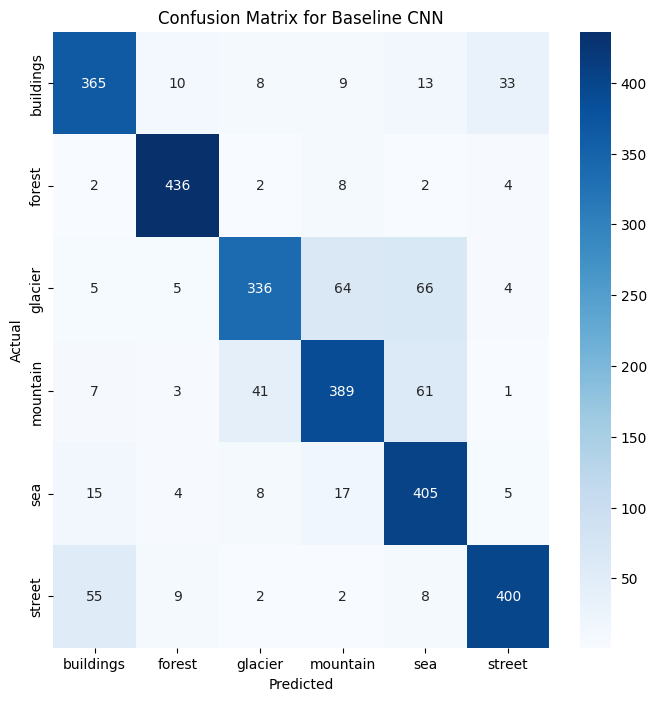
The confusion matrix confirmed the model was great at spotting “forests,” but it put a bright spotlight on our key problem: it misclassified 65 “glacier” images as “mountain” and 52 “mountain” images as “glacier”. The antagonist was real.
Act II: Getting smarter with regularization (88% accuracy)
The baseline model was good, but I had a nagging fear of overfitting. Was it truly learning or just memorizing? I built a deeper, four-block CNN and integrated a suite of regularization techniques to help it generalize better.
Batch normalization: a recipe for stability. This is a technique that standardizes the inputs to a layer for each mini-batch, ensuring the data distribution remains consistent. Think of a long assembly line for baking cakes; batch normalization is like placing a quality control expert at each station who standardizes the batter before passing it on, making the whole training process faster and much more stable.
Dropout: forcing teamwork. This technique randomly sets a fraction of neuron activations to zero during each training step, preventing any single neuron from becoming too specialized. Dropout is like a coach who, during each practice drill, tells random players to sit out for that play, forcing the remaining players to work together and making the team as a whole much stronger.
Early stopping: the wise proctor. This method involves monitoring the model’s performance on a validation set and stopping the training if the performance stops improving. We were already using this, but it’s worth highlighting again; Early stopping is the wise proctor who watches the model’s performance and stops the training the moment its scores start getting worse, preventing it from “over-studying.”
Here’s a look at the more complex architecture.

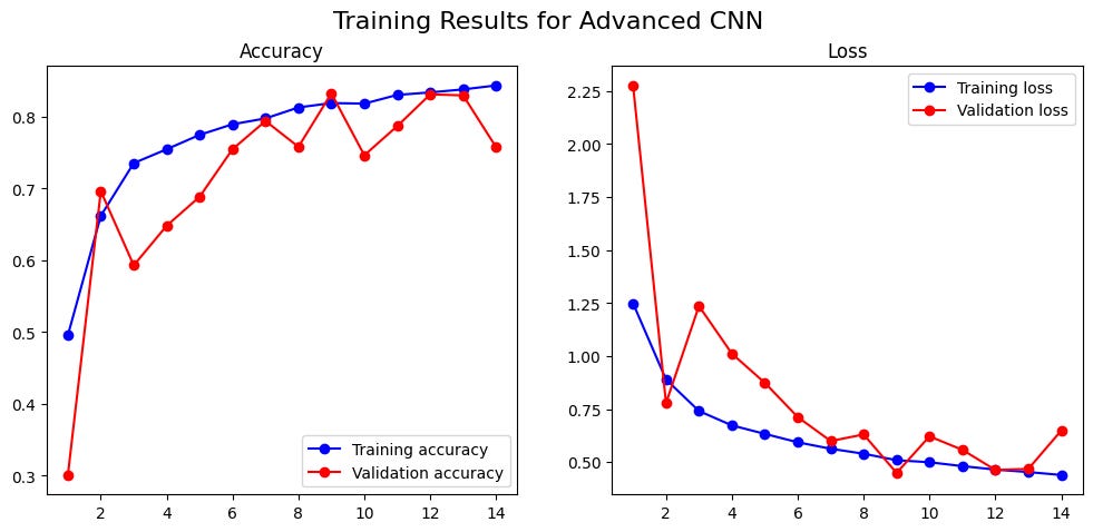
This new model was a significant upgrade. Instead of two feature-finding blocks, it had four. It started with 32 filters, then progressively deepened to 64, 128, and finally 256 filters, allowing it to learn much more abstract and complex patterns. Each block was a sandwich of Conv2D layers followed by BatchNormalization for stability and a MaxPooling2D layer for summarization. Crucially, a Dropout layer was added after each block to force the network to learn more robust features. For the classification head, I replaced the simple Flatten layer with a more modern GlobalAveragePooling2D layer, which is more efficient and less prone to overfitting. This was followed by a heavily regularized set of Dense layers to make the final prediction.
The results were immediate: 88% accuracy. However, the training curves showed considerable volatility, with the validation loss spiking erratically. This proved a key lesson: deeper, more complex models can be much harder to train.
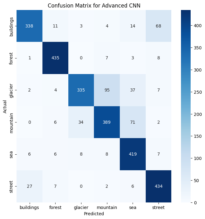
But to see exactly where we improved, we once again turned to the confusion matrix, comparing it directly to our baseline. The new matrix showed we were making real progress on the glacier-mountain problem, with the number of misclassifications dropping. The smarter training techniques were clearly helping the model learn more effectively.
Act III: Standing on the shoulders of giants (93% accuracy)
88% was good, but building from scratch felt like re-inventing the wheel. What if we could leverage the work of top research labs? This is the core idea behind transfer learning. The analogy I love is learning the ukulele after playing classical guitar: you transfer your knowledge of chords and music theory to learn much faster.
In my case, the “giants” whose shoulders we’d be standing on are powerful, pre-trained models that have already learned to recognize fundamental visual patterns from the massive ImageNet dataset. I decided to pit three famous architectures against each other to see how they’d fare on our specific problem.
VGG16, the reliable veteran: Developed by the Visual Geometry Group at the University of Oxford around 2014, VGG16 is a classic. It’s known for its straightforward, deep architecture that exclusively uses small 3x3 filters. It’s a solid, reliable performer: the dependable workhorse of the deep learning world.

ResNet50, the complex powerhouse: Introduced by Microsoft Research in 2015, ResNet was a revolutionary breakthrough. Its key innovation is the “residual” or “skip connection,” which allows the network to learn to skip layers if they’re not useful. This clever trick allows for the creation of incredibly deep networks (50 layers in this case) without the performance degrading, making it a theoretically more powerful architecture.

EfficientNetB0, the modern champion: Hailing from Google in 2019, EfficientNet represents a more modern approach. Instead of just making networks deeper, it uses a principled method to balance network depth, width, and image resolution. It was designed to be both highly accurate and computationally efficient, making it a state-of-the-art champion for many tasks.
With the contenders chosen, the experiment began.
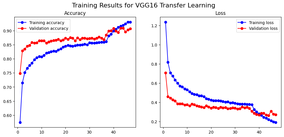
VGG16 (91% accuracy): I loaded the pre-trained VGG16, froze its layers, and trained our own small “head.” Then, we unfroze the top few layers of the base and continued training with a very low learning rate. The training was incredibly stable, and the result was a stunning 91% accuracy.
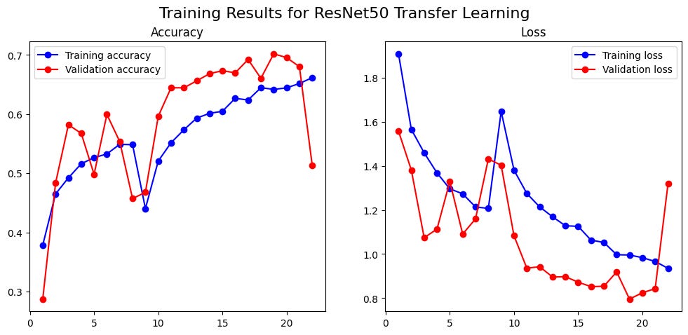
ResNet50 (70% accuracy): I expected this more modern architecture to do even better. It failed. Spectacularly. The training was highly volatile, topping out at a dismal 70%. It was a powerful reminder that theoretical complexity doesn’t guarantee superior performance.
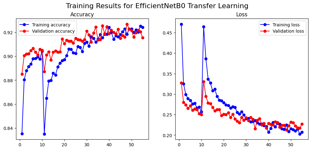
The Champion: EfficientNetB0 (92.94% Accuracy) This state-of-the-art model, paired with an even more aggressive data augmentation strategy, delivered the best performance: a phenomenal 92.94% accuracy. It excelled where others struggled, making it the champion.
The debrief: analysis, trust, and takeaways
We had our champion model. But as a PM, I needed more than a number. I needed to understand why it worked. We needed to peek inside the black box.
Peeking inside the black box with Grad-CAM
To understand a model’s decision-making process, I used Grad-CAM. It’s like giving your model a highlighter. It generates a “heatmap” over the original image, showing you the pixels that were most influential in its decision.
This isn’t just a cool visualization. It’s a critical tool for debugging, identifying bias, and building stakeholder trust. With the simple Baseline CNN, Grad-CAM was incredibly insightful. When the model made a mistake, the heatmap would clearly show why.
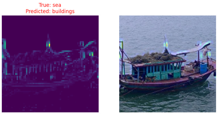
Take the example above. The baseline model looked at an image that was clearly in the ‘sea’ category and incorrectly predicted ‘buildings’. At first, that seems like a bizarre error. But the Grad-CAM heatmap instantly explains the model’s logic. The bright yellow spots show that the model completely ignored the water and the boat, and instead focused its entire attention on the architectural structures in the background. It wasn’t a random guess; it was a logical mistake based on the features it had learned to prioritize.
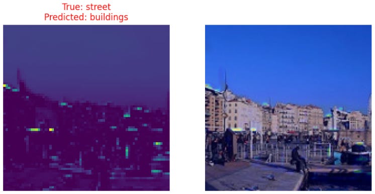
Here’s another one. The model misclassified this “street” scene as “buildings.” Again, the heatmap tells the story. The model’s attention is almost exclusively on the row of building facades, ignoring the street, the people, and the waterfront. This kind of insight is invaluable for a PM because it turns a mysterious error into a concrete product discussion about feature engineering and potential data biases.
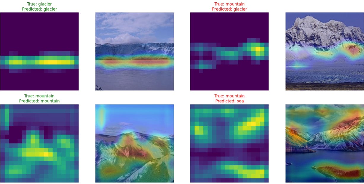
However, one of the most surprising “aha moments” of the project was discovering that as the models became more accurate and complex, they also became harder to interpret. I expected the Grad-CAMs for our advanced models to be sharper, but often the opposite was true. With hundreds of complex filters at work, the heatmaps became more diffuse and difficult to decipher. The model was seeing something the right way, but its reasoning was distributed across so many layers that it was no longer simple for a human to understand at a glance.
Here is a Grad-CAM for the advanced CNN:
And this one for EfficientNetB0:
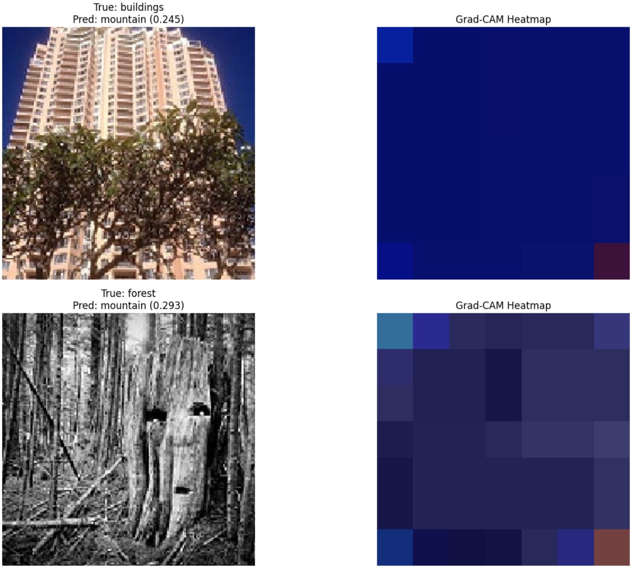
This revealed a critical product trade-off: sometimes, higher accuracy comes at the cost of lower interpretability. The “black box” can actually get “blacker” as it gets smarter. This is a crucial consideration for any PM. Do we ship the 93% accurate model that nobody can explain, or the 88% model that we can easily debug when it fails? The answer depends entirely on your product and your users’ tolerance for opaque decision-making.
A quick detour: how pros find the best settings
In this project, I mostly used established practices to set the hyperparameters. But in a professional setting, you’d be more rigorous using techniques like:
Grid search: An exhaustive search through a manually specified list of hyperparameter combinations to find the best one.
Cross-validation: A robust technique to evaluate a model by splitting the data into multiple “folds” and training/testing the model on different combinations of those folds to ensure the results are consistent.
Lessons for your next AI product
I successfully went from an 83% MVP to a 93% state-of-the-art champion. This wasn’t a single breakthrough but a systematic, iterative process of building, measuring, and learning: a cycle familiar to any product manager.
If you remember nothing else from this journey, remember these three lessons:
Find the right trade-off: from baseline to state-of-the-art. Building a simple baseline model is an invaluable first step. It proves the concept is viable and gives you a benchmark. While transfer learning is the north star for achieving high performance, the ultimate goal isn’t always the highest possible accuracy. As a PM, your job is to deliver what is “good enough” to solve the user’s problem effectively. An 88% accurate model that is highly interpretable and can be supplemented with a Human-in-the-Loop (HITL) system might be a far better product than a 93% accurate “black box” that took twice as long to build.
Complexity is a risk, not a virtue: The ResNet50 failure is your cautionary tale. Always question if adding complexity is worth the risk. Sometimes, the reliable workhorse is better than the temperamental racehorse.
Demand interpretability (and understand its limits): Don’t settle for just an accuracy score. Ask your data science team for the confusion matrix and Grad-CAM outputs. But also be aware that as models get better, they may get harder to explain. This trade-off between accuracy and interpretability is a key strategic decision you’ll need to make.
Building an AI product isn’t about finding a single magic algorithm. It’s about a disciplined, curious, and story-driven journey from a simple question to an intelligent solution. By understanding the key trade-offs, asking the right questions, and demanding transparency, you can lead your team not just to a high accuracy score, but to a product that truly delivers value and earns your users’ trust. And in the end, it’s still magical that we can call on all this complex math and computational power with just a few lines of code.
This was my journey into the world of deep learning, but every PM’s path with AI is different. What’s your experience been? Have you taken on a side project to learn a new technical skill, or have you found other ways to bridge the gap with your engineering team? I’d love to hear your stories and what’s worked for you.
I’m going to mention a problem that’s similar to what https://www.quora.com/profile/Haohan-Wang mentioned, but with a different twist:
Why does deep learning generalize so well, despite using parameters that are orders of magnitude more numerous than the training samples?
Let me give you an example. Consider the https://arxiv.org/pdf/1409.1556.pdf deep convolutional neural net that won the ImageNet challenge in 2014 (in classification+localization category). It has upwards of 130 million parameters and still performs amazingly well on a puny dataset like the https://www.cs.toronto.edu/~kriz/cifar.html which only has 60,000 thumbnail sized images!
Let me repeat. The algorithm has 130 million tunable parameters! That is enough parameters to memorize the entire CIFAR-10 dataset bit by bit a hundred times over! But somehow VGG19 doesn’t overfit and actually gives a decent test accuracy! How in the world is it doing that?
Now compare that to a typical “non-deep” machine learning algorithm like the logistic regression. For CIFAR-10’s 32x32 color images, the number of parameters would be just over 3,000. Even if you add polynomial features of order up to 10 for every pixel of every color (which will lead to terrible overfitting), the parameter count is still thousands of times lower than VGG19!
Conventional deep learning techniques that are used to prevent overfitting (like dropout, L1 regularization, L2 regularization etc.) don’t even come close to offering a convincing explanation for this mysterious phenomenon. There is a lot to be understood.
Excellent !!