How to convert massive raw data into an AI graph

A hands-on experiment transforming the 4GB Yelp dataset into structured intelligence with Neo4j. We cover everything from batch ingestion and configuration hacks to building AI-powered recommendation.

Many thanks to my professor at Sorbonne University, Ansoumana Cissé, for his excellent course and for suggesting this very project.

---

We need to talk about the Excel view of the world. As product managers, we are trained to think in tables. We have a Users table. We have a Orders table. If we want to know what a user bought, we mentally draw a line between Row 4 in one sheet and Row 12 in another. We treat products, customers, and data as isolated islands, sitting in rigid, square cells.

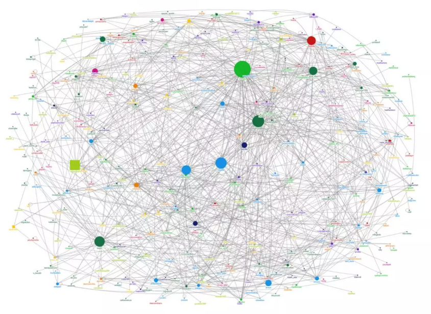
But that is not how the world works. And it is certainly not how advanced companies structure their data. Years ago, I saw this slide from Netflix explaining their data architecture that changed how I see data. When they visualize their ecosystem, it doesn’t look like a spreadsheet. It looks like a constellation. It’s a spectacular, messy, interconnected galaxy where an Asset is linked to a Movie, which is linked to a Display Set, which is linked to a User who watched it on a Tuesday.

Netflix’s digital asset management graph model (source)

They don’t just store data; they store relationships.

This highlighted a disconnect in how many of us build AI-powered products today. We want AI to be associative, to connect the dots like a human brain, but we store those dots in separate, rigid boxes.

To understand this architectural shift better, especially as I work on AI initiatives, I wanted to gain first-hand experience. I realized that the best way to understand why a graph might be better than a standard SQL table for AI was to move beyond theory and actually use the technology. So I decided to conduct an experiment using the Yelp Open Dataset, a massive collection of over 4GB of Businesses, Users, Reviews, Tips, and Check-ins. My goal was to ingest this data into Neo4j and see if I could build working graph databases on my laptop.

This article documents the complete end-to-end experiment. From the theoretical basics to the nitty-gritty of execution, here is the path we will take to turn 4GB of raw JSON into a living, thinking graph:

• What is Neo4j? Understanding why we need to move beyond thinking in tables.

• The setup: Configuring a local instance and preparing the environment.

• Data integration: Strategies for ingesting millions of records without crashing the system.

• The sanity check: Verifying the plumbing and relationships before running complex queries.

• The analysis: Stress-testing the graph with 10 queries, moving from simple statistics to complex pattern discovery.

• The recommendation engine: Prototyping content-based, collaborative, and hybrid algorithms.

• Going further: Using Graph Data Science (GDS) to uncover hidden social structures.

• The reality: The actual technical hurdles, from memory walls to config hacks, encountered along the way.

• The verdict: Is Neo4j worth the hype?

Ready to explore what happens when we finally connect the data?

---

The fundamentals: what is Neo4j?

When you dig into how companies like LinkedIn map your “2nd degree connections” or how Amazon determines “frequently bought together” items, you keep hitting the same concept: the graph database. And in that world, Neo4j is the heavyweight champion.

Founded in the 2000s by Emil Eifrem, who actually coined the term “graph database,” Neo4j is to graphs what Google is to search. It is the market leader, but it is certainly not the only player in town. Here are three key alternatives worth knowing:

• Amazon Neptune: A managed graph service that integrates with other AWS tools.

• ArangoDB: A multi-model database that handles graphs, documents (JSON), and key-values all in one place.

• TigerGraph: Known for its focus on massive parallel processing, often used for heavy analytics on huge datasets.

So why focus on Neo4j? For a product manager or anyone starting their journey, Neo4j is the standard. It has the largest community, the most documentation, and it feels the most approachable for beginners. More importantly, it is currently leading the charge in the intersection of graphs and generative AI.

We know that LLMs have a flaw: they hallucinate. They don’t know facts; they predict the next likely word. To fix this, the industry is moving toward GraphRAG. Instead of feeding an LLM a flat text document, you feed it a knowledge graph, a structured map of true relationships. Neo4j has effectively evolved into the memory layer for AI, allowing models to think by hopping from concept to concept, just like a human brain, rather than scanning millions of rows of text.

To understand why a graph architecture is different, you don’t need to read code. You just need to understand the difference between a join and a pointer.

Relational joins vs. graph pointers

• The relational model, the spreadsheet way: Imagine you want to find “friends of friends” in a standard SQL database (like MySQL or Postgres). Data lives in separate tables. To connect a User to their Friends, the database has to perform a JOIN. It takes the user’s ID, goes to an index (like the back of a textbook), looks up the location of the friend, and then jumps to that table. It does this for every single connection. As your data grows, these hops get exponentially expensive. It’s like trying to trace a family tree, but for every relative, you have to drive back to the city archives to find their address.

• The graph model, the Neo4j way: In a graph, there are no tables. There are only nodes (the nouns) and relationships (the verbs). Alice is a Node. Bob is a Node. The connection [:IS_FRIENDS_WITH] is a physical pointer connecting them in memory. To find “friends of friends,” the database doesn’t look up an index. It simply “walks” from Alice to Bob to Charlie. It’s instantaneous. In engineering terms, this is called index-free adjacency.

For the AI use cases we care about (recommendation, personalization, and context) relationships are not just metadata; they are the most valuable part of the dataset.

The real payoff of this pointer architecture is scalability. In the SQL world, you inevitably hit the O(n) problem: as your tables grow, your indexes grow, and join operations get progressively slower because the database has to scan more data. You effectively pay a performance tax for every new row you add. Neo4j avoids this tax completely. Because it follows direct memory pointers, traversing a relationship takes the same amount of time whether your database has a thousand nodes or a billion. The performance depends only on the specific subgraph you are exploring, not the total volume of data stored.

That is enough theory. Let’s move to the practice.

---

The setup: local vs. cloud

Before starting the project, I had to make an infrastructure decision: where does this graph live? In the Neo4j ecosystem, there are two main paths:

• The first is Neo4j AuraDB, a fully managed cloud service. This is the happy path: it handles backups, updates, and scaling for you. For a company building a production product, this is the obvious choice.

• The second path is Neo4j Desktop, a local application you install on your machine. This is the hacker path. It gives you total control over the database configuration, lets you manipulate memory settings, and runs entirely offline.

For this project, I made a trade-off: While the cloud is easier, the free tier has strict limits on graph size. Since I planned to ingest the massive Yelp dataset (over 10 million nodes and relationships), running this in the cloud would likely require a paid tier. I chose Neo4j Desktop to avoid costs and, more importantly, to force myself to manage the hardware constraints directly.

If you want to follow along with this project, I recommend starting locally so you don’t hit cloud limits with the large Yelp dataset.

There are four main steps to getting your local environment ready:

Steps required to get your local Neo4j environment up and running

• Step 1: Download the tool. Go to the Neo4j Download Center and download Neo4j Desktop. It’s free for personal use.

• Step 2: Create a local instance. Once you open the app, you need to create a new instance. Click on Create instance. You will be asked to name your instance (I called mine “YelpProject”) and define a password. Important: Write this password down. You cannot recover it easily, and you will need it every time you connect.

Creating a new local Neo4j instance is as simple as naming it and setting a password

• Step 3: Install the plugins. We need to install two critical plugins: think of these as the Excel macros of the graph world:

  • APOC (Awesome Procedures on Cypher): A utility library that lets us import complex JSON files.

  • GDS (Graph Data Science): The powerhouse library containing the AI algorithms like PageRank.

  Click on your new instance (don’t start it yet), go to the Plugins tab on the right, and click Install for both APOC and Graph Data Science Library.

The “Plugins” tab showing APOC and GDS installed

• Step 4: Start the engine. Click Start. It might take a few seconds to initialize the graph engine. Once the status turns green, the empty graph brain is ready to learn.

Once the instance status shows “Running,” the database is active and ready for data ingestion.

The infrastructure is built. Now, we need a dataset worthy of it!

---

The data: from JSON to graph

For this experiment, I didn’t want to play with a toy dataset of 50 rows. I wanted real-world chaos. I chose the Yelp Open Dataset, a massive 4GB+ collection of user-generated content.

The Yelp Open Dataset offers a massive, real-world sandbox (4GB+) for testing graph algorithms

Functionally, Yelp is simple: Users write Reviews for Businesses. But structurally, it is rich with context. It includes Tips (short timestamps), Check-ins (traffic signals), and Categories (taxonomies).

If this were a SQL project, I would be worrying about foreign keys and join tables. In Neo4j, I just had to visualize the sentence:

A User WROTE a Review about a Business.

That sentence became my schema:

(User)-[:WROTE]->(Review)-[:REVIEWS]->(Business)

To make this schema a reality, we use Cypher, Neo4j’s query language. Invented in 2011 by Andrés Taylor, an engineer at Neo4j, Cypher was designed to solve a specific pain point: SQL is terrible at describing connections. In SQL, if you want to find “friends of friends,” you have to write complex JOIN statements that are hard to read and slow to run.

Cypher is different because it is declarative and visual. It was inspired by ASCII art, the way engineers used to draw diagrams in code comments.

The basic rules of Cypher are:

• Nodes are circles: (u:User) looks like a circle.

• Relationships are Arrows: -[:WROTE]-> looks like an arrow.

• Properties are JSON-like: {name: “Ed”} adds detail.

So, instead of writing 10 lines of SQL Joins, you just draw the pattern you want to match: (User)-[:WROTE]->(Review)

As a product manager, you don’t need to be a syntax expert to use Cypher; you just need to be a logic expert. Because the code looks like the whiteboard diagram, the gap between product requirement and database query disappears.

For my part, I didn’t even write the code from scratch. I prompted Gemini: “Here is the JSON structure of the Yelp dataset. Write me a Cypher import script to create nodes and relationships.” I was genuinely surprised by how effective Gemini was at writing this specific language. Even though Cypher is less common than SQL, Gemini generated scripts that work. This bridge allows anyone to focus on the logic of the graph without getting stuck on syntax errors. By the way, if you want to get up to speed quickly, just ask Gemini for a “Cypher cheat sheet,” it is the perfect primer to help you read and verify the scripts before you run them.

Let’s get back to our use case. When you unzip the Yelp Open Dataset, you aren’t just greeted by data. You get a PDF documentation file explaining the structure. Inside, you will find several massive JSON files. We don’t need everything. We need to focus on the three files that form the core of the Yelp experience:

• yelp_academic_dataset_business.json: This lists the places. It contains the business_id, name (e.g., “Garaje”), city, and crucially, categories. In the raw JSON, categories appear as a string list like “Mexican, Burgers, Gastropubs”. In our graph, we won’t just store this as text; we will split them into separate Category nodes so we can find connections between different restaurants.

• yelp_academic_dataset_user.json: This lists the people. It contains the user_id, name, and their social network stats.

• yelp_academic_dataset_review.json: This is the connector. It bridges the gap, containing a user_id (who wrote it), a business_id (who it is about), the stars, and the text.

We have the raw JSON files, but how do we structure them? The beauty of graph modeling is that the schema often mirrors plain English. To define the connections, I simply visualized the core interaction of the platform:

A User WROTE a Review about a Business that is IN_CATEGORY a Category.

That simple sentence became my schema. Instead of tables, we define Nodes (the nouns) and Relationships (the verbs).

The target schema: Mapping data into four nodes (User, Review, Business, Category) linked by action-oriented relationships

With this blueprint in mind, we can move to the practical steps.

Steps required for the data ingestion process

• Step 1: Get the data. Download the JSON version of the Yelp Open Dataset. Unzip it. You will see huge files like yelp_academic_dataset_review.json.

• Step 2: The “import” folder. Neo4j Desktop has a strict security feature: it can only read files from a specific folder.

  • Hover over your Project name in Neo4j Desktop.

  • Click the three dots (...) → Open → Instance folder.

  • Drag your JSON files into this folder.

You must open the specific “Instance folder” via the database menu to add files

Drag and drop your unzipped Yelp JSON files directly into the import directory within that folder

• Step 3: The constraints. Before we load data, we must tell the database what makes a node unique. If we don’t, Neo4j will scan the entire database every time we add a user to check if they already exist. This is slow. Run this Cypher code in the query bar to create unique constraints: think of these as the bouncers at the door checking IDs.

CREATE CONSTRAINT FOR (b:Business) REQUIRE b.id IS UNIQUE;
CREATE CONSTRAINT FOR (u:User) REQUIRE u.id IS UNIQUE;
CREATE CONSTRAINT FOR (r:Review) REQUIRE r.id IS UNIQUE;
CREATE CONSTRAINT FOR (c:Category) REQUIRE c.name IS UNIQUE;

Defining unique constraints is the critical step that ensures data integrity and speeds up the import process

• Step 4: The batch import. This was my first big hurdle. If you try to load 4GB JSON files in one go, your RAM will overflow, and Neo4j will crash. The solution is to use the APOC plugin we installed earlier. Specifically, we use a function called apoc.periodic.iterate. Think of this as a factory conveyor belt: instead of dumping the whole truckload of data onto the floor at once, it processes the data in small batches (e.g., 10,000 records at a time). This keeps the memory usage low and stable. We need to import the data in a specific order: first the nouns (Businesses, Users), and then the verbs (Reviews) that connect them.

Time to load. We will run these scripts one by one. When you execute them, you won’t see a live counter, just a loading spinner. Be patient. When it finishes, you will see a result table confirming the number of batches processed. Once you see the green checkmark, you are safe to move to the next step.

1. Importing Businesses (and Categories). First, we create the places. The Yelp dataset hides categories (like “Mexican” or “Bar”) inside the Business file as a comma-separated string. We need to split that string and create distinct Category nodes on the fly.

CALL apoc.periodic.iterate(
  “CALL apoc.load.json(’file:///yelp_academic_dataset_business.json’) YIELD value RETURN value”,
  “MERGE (b:Business {id: value.business_id})
   SET b.name = value.name,
       b.address = value.address,
       b.city = value.city,
       b.state = value.state,
       b.stars = value.stars,
       b.review_count = value.review_count,
       b.is_open = value.is_open
   WITH b, value
   WHERE value.categories IS NOT NULL
   UNWIND split(value.categories, ‘, ‘) AS catName
   MERGE (c:Category {name: catName})
   MERGE (b)-[:IN_CATEGORY]->(c)”,
  {batchSize: 10000, parallel: false}
);

Importing 150,000+ businesses and unwinding their categories into connected nodes took about 17 seconds

2. Importing Users: Next, we import the people. This is a larger file (nearly 2 million users), so the batching strategy is critical here. We map the user_id and their name.

CALL apoc.periodic.iterate(
  “CALL apoc.load.json(’file:///yelp_academic_dataset_user.json’) YIELD value RETURN value”,
  “MERGE (u:User {id: value.user_id})
   SET u.name = value.name,
       u.review_count = value.review_count,
       u.yelping_since = value.yelping_since,
       u.average_stars = value.average_stars”,
  {batchSize: 10000, parallel: true}
);

Successfully processing nearly 2 million User profiles using a batch size of 10,000 to manage memory

3. Importing Reviews (the connector). This is the heavy lifting. The Review file contains nearly 7 million records. For every single review, the database has to:

• Find the User (who wrote it).

• Find the Business (being reviewed).

• Create the Review node.

• Draw the arrows: (User)-[:WROTE]->(Review)-[:REVIEWS]->(Business).

CALL apoc.periodic.iterate(
  “CALL apoc.load.json(’file:///yelp_academic_dataset_review.json’) YIELD value RETURN value”,
  “MATCH (u:User {id: value.user_id})
   MATCH (b:Business {id: value.business_id})
   MERGE (r:Review {id: value.review_id})
   SET r.stars = value.stars,
       r.date = value.date,
       r.text = value.text,
       r.useful = value.useful,
       r.funny = value.funny,
       r.cool = value.cool
   MERGE (u)-[:WROTE]->(r)
   MERGE (r)-[:REVIEWS]->(b)”,
  {batchSize: 5000, parallel: false}
);

The final and largest step: ingesting 6.9 million reviews and linking them to users and businesses took about 8 minutes

• Step 5: Verify the graph. Once the loading bars finish, you need to verify the connections. Run a simple query to visualize the schema.

CALL apoc.meta.stats() YIELD labels, relTypesCount

The moment of truth: verifying that 6.9 million Reviews are correctly connected to Users and Businesses.

Mission accomplished. If you see green checkmarks across the board, you have successfully built a professional-grade graph database on your laptop. We now have roughly 150,000 Businesses, 1.98 million Users, and 6.99 million Reviews living in our system. Note: We will discuss the specific ingestion challenges I faced in a dedicated section.

Now that the data is loaded, let’s verify that the connections actually work!

---

The sanity check: first contact with the graph

Before running complex queries or trying to build a recommendation engine, I needed a “hello world” moment. Let’s verify that the schema wasn’t just a drawing on a whiteboard, but a reality in the database.

Verification 1: The unbroken chain unit test. My first goal was to confirm that the data loaded correctly and that the relationships actually connected across the entire schema. I wanted to find one single, continuous path starting from a User and ending at a Category.

Run this query in Neo4j. Switch to the graph view so you see the connected circles.

MATCH path = (u:User)-[:WROTE]->(r:Review)-[:REVIEWS]->(b:Business)-[:IN_CATEGORY]->(c:Category)
RETURN path
LIMIT 1;

A single “Unbroken Chain” verifying the data model. This path connects User “Erin” to a Review, which connects to the Business “Abby Rappop…,” finally landing on the Category “Doctors”

This single chain perfectly mirrors the target schema we designed earlier. It visually confirms that the theoretical model (User connecting to Review, Review to Business, and Business to Category) is now a functional reality in the graph.

Don’t just look at the shapes: interact with them. Click on any node (like a Business or User) or even a relationship arrow (like WROTE) in the graph visualization. The side panel will slide open. It reveals the actual data stored inside. This is the opportunity to verify that properties like address, stars, and city were correctly parsed from the JSON files and attached to the right entities.

By clicking on the Business node in the path, I confirmed that all properties, like Address, Stars, and City, were correctly parsed from the JSON and stored in the node

Verification 2: The visual cluster. Once I knew the basic path existed, I wanted to see the network in action. I ran a broader query to visualize a cluster of Users, their Reviews, and the Businesses they talked about.

MATCH (u:User)-[:WROTE]->(r:Review)-[:REVIEWS]->(b:Business)
WITH u, r, b
LIMIT 50
RETURN u, r, b

This query returns a small subgraph that lets you verify the density of connections. You should see clear chains flowing from User to Review to Business.

Visualizing the local network: A cluster of 50 connected nodes showing the flow from Users to Reviews to Businesses

A helpful tip when exploring this view is to double-click on any Business circle. This expands the node to reveal other users who have reviewed that same location, instantly showing you the “community” around a specific place.

Double-clicking a Business node instantly reveals the surrounding community of users who reviewed it

With the structure verified and the plumbing confirmed, we are ready to leave the engineering phase behind. Now, let’s stress-test our new graph with 10 queries, moving from simple statistics to complex pattern discovery.

---

The analysis: 10 queries to play with the graph

Now, imagine you have the entire Yelp ecosystem, 10 million nodes of chaos, living on your laptop. The data isn’t just stored in rows anymore; it is connected. This is where the fun begins. In a SQL database, exploring this level of depth usually means writing complex, painful JOIN queries. In Neo4j, it feels more like interviewing your data.

And the best part? I didn’t write these queries from scratch. I treated Gemini as a junior data engineer. I simply asked plain English questions like “How do I find the most active users?” or “Show me the review trends over time,” and it generated the Cypher code for me.

Here are the 10 queries we used to explore the richness of the graph.

1. What are the top 10 most common business categories? This is a simple aggregation to see what dominates the dataset.

MATCH (c:Category)<-[:IN_CATEGORY]-(b:Business)
RETURN c.name AS category, count(b) AS business_count
ORDER BY business_count DESC
LIMIT 10;

A simple aggregation reveals the dominant categories in the Yelp dataset, with “Restaurants” taking the top spot by a wide margin

2. Who are the super users? Finding the 10 users who have written the most reviews.

MATCH (u:User)-[:WROTE]->(r:Review)
RETURN u.name AS user_name, count(r) AS review_count
ORDER BY review_count DESC
LIMIT 10;

Identifying the super users: the individuals who have contributed the highest volume of reviews to the platform

3. The cream of the crop. Finding the 10 best-rated businesses, but filtering for those with at least 100 reviews to ensure reliability.

MATCH (b:Business)
WHERE b.review_count > 100
RETURN b.name AS business_name, b.stars AS average_rating, b.review_count
ORDER BY average_rating DESC
LIMIT 10;

Filtering for quality and reliability: Finding the cream of the crop businesses that maintain a perfect 5-star rating across hundreds of reviews

4. How has the volume of reviews evolved over time? A temporal analysis to see the platform’s growth year over year.

MATCH (r:Review)
RETURN toInteger(left(r.date, 4)) AS year, count(r) AS review_count
ORDER BY year;

A temporal analysis showing the platform’s explosive growth, with review volume doubling nearly every year in the early days

5. The toughest critics. Instead of looking for popularity, let’s look for the users who are hardest to please. These are experienced users (>50 reviews) with the lowest average ratings.

MATCH (u:User)
WHERE u.review_count > 50 
RETURN u.name AS user_name, u.average_stars AS avg_rating, u.review_count
ORDER BY avg_rating ASC
LIMIT 10;

Identifying the platform’s toughest critics: Experienced users (>50 reviews) who maintain incredibly low average ratings, some as low as 1.01 stars

6. The novelists: longest reviews. Who writes the longest essays? This query calculates the character count of reviews to find the most detailed contributors.

MATCH (r:Review) 
RETURN substring(r.text, 0, 50) + “...” AS preview, size(r.text) AS length 
ORDER BY length DESC 
LIMIT 5;

Finding the novelists: A query sorting reviews by character count reveals users hitting the 5,000-character limit with their feedback

7. The category explorers. Most users stick to one lane (e.g., only reviewing restaurants). This query finds the users with the most diverse tastes, reviewing the widest variety of unique categories.

MATCH (u:User)-[:WROTE]->(:Review)-[:REVIEWS]->(:Business)-[:IN_CATEGORY]->(c:Category) 
RETURN u.name, count(distinct c) AS diverse_tastes 
ORDER BY diverse_tastes DESC 
LIMIT 10;

Uncovering category explorers: Users with the most diverse tastes, traversing over 1,100 distinct business categories in their review history

8. The local experts. This looks for users who have hyper-local knowledge, those who have reviewed the most businesses within a single city.

MATCH (u:User)-[:WROTE]->(:Review)-[:REVIEWS]->(b:Business) 
RETURN u.name, b.city, count(b) AS local_reviews 
ORDER BY local_reviews DESC 
LIMIT 10;

Spotting local experts: Users who demonstrate hyper-local knowledge by contributing thousands of reviews within a single city, like Philadelphia.

9. Finding hidden gems. We often look for the most popular spots, but what about the underdogs? This query finds businesses with high ratings (4.5+) but a low review count (10-50).

MATCH (b:Business)
WHERE b.stars >= 4.5 AND b.review_count > 10 AND b.review_count < 50
RETURN b.name, b.stars, b.review_count
ORDER BY b.review_count ASC
LIMIT 10;

Discovering hidden gems: Businesses that maintain high quality (4.5+ stars) but haven’t yet been flooded with reviews (low count)

10. The elite hangouts. Instead of following the crowd, where do the power users go? This query filters for users with over 1,000 reviews and maps their most frequent spots. This is a great way to find places that are expert approved.

MATCH (u:User)-[:WROTE]->(:Review)-[:REVIEWS]->(b:Business)
WHERE u.review_count > 1000
RETURN b.name, b.city, count(u) AS vip_visits
ORDER BY vip_visits DESC
LIMIT 10;

Mapping elite hangouts: Filtering for users with 1,000+ reviews reveals exactly where the platform’s elites actually eat

Warm-up is over. If you are a SQL veteran, you might be looking at these queries and thinking, “I could have done most of this with a few joins.” And you wouldn’t be wrong. But we didn’t load 10 million nodes just to do simple aggregation. Now, let’s get serious. It is time to stop querying the past and start predicting the future. Let’s bring actual algorithms into the game.

---

The feature: building recommendation prototypes

We have ingested the data and explored the patterns. Now, it is time to switch hats from data analyst to product builder. My goal wasn’t to build a production-grade engine overnight, but to prototype three different ways to answer a simple user problem: “Where should I eat tonight?”

To do this, I asked Gemini to design three distinct algorithms. But before we look at the code, we need to agree on the strategy. In the world of recommender systems, there are three main schools of thought. Here is the logic we are choosing between:

Visualizing the three logic models: the librarian matches attributes, the friend matches people, and the expert combines both for the best results

1. Content-based filtering, the librarian. This approach relies on attributes. It looks at the metadata of what you liked (e.g., “Mexican,” “Cheap,” “Downtown”) and finds other items with the exact same tags. It’s like a librarian saying, “Oh, you enjoyed this mystery novel set in Victorian London? Here is another mystery novel set in Victorian London.” The trade-off: It is safe and highly explainable, but it creates a filter bubble. You will never discover a great sushi place if you only keep asking for more tacos.

2. Collaborative filtering, the friend. This approach relies on behavior. It ignores the tags and looks at the people. It finds users who are taste twins (people who liked the same things you did) and recommends what they liked that you haven’t seen yet. It’s like a friend saying, “Hey, we usually love the same restaurants, and I just went to this crazy new Korean BBQ spot. You have to try it.” The trade-off: It creates Serendipity (finding things you wouldn’t naturally search for), but it suffers from the cold start problem. If you don’t have enough data to find a twin, the system fails.

3. Hybrid filtering, the expert. This combines both. It uses collaborative filtering to find popular, high-quality spots approved by your peers, but filters them through content-based logic to ensure they actually match your specific preferences. It’s like a local expert saying, “People with your taste profile absolutely love this place, AND it happens to serve the specific type of spicy food you’re looking for right now.” The trade-off: This is the gold standard, balancing relevance with discovery, but it is the most complex to build.

Now that we have the strategy, let’s start with the simplest approach: the Librarian.

Prototype 1: Content-based filtering, the Jaccard index

The concept: Imagine a user is looking at the page for “Tsevi’s Pub And Grill.” They scroll down to the “You might also like” section of Yelp. Our goal is to fill that section with businesses that are structurally similar: places that have the exact same DNA (Categories) as the original spot.

The logic: Gemini suggested using the Jaccard Index. For a product manager, think of this as a “Venn Diagram Score.”

The Jaccard index explained

• If two restaurants have identical categories (100% overlap), the score is 1.0.

• If they share nothing (0% overlap), the score is 0.0.

• Why not just count shared tags? Because a place with 50 tags would match everything. Jaccard is smarter: it measures the ratio of shared tags, ensuring a fair comparison between a simple dive bar and a complex resort.

The query: We are calling the Graph Data Science (GDS) library directly in the query (gds.similarity.jaccard). This function handles the heavy math for us. Note that we are running this analysis specifically for one target business (“Tsevi’s Pub And Grill”) to find its direct siblings, rather than calculating similarities for the entire database at once.

// 1. Find the target business and its categories
MATCH (b1:Business {name: “Tsevi’s Pub And Grill”})-[:IN_CATEGORY]->(c:Category)
WITH b1, collect(id(c)) AS b1_category_ids

// 2. Compare it against every other business
MATCH (b2:Business)-[:IN_CATEGORY]->(c2:Category) WHERE b1 <> b2
WITH b1, b1_category_ids, b2, collect(id(c2)) AS b2_category_ids

// 3. Calculate Jaccard Similarity and return top 10
RETURN b2.name AS recommendation, 
       gds.similarity.jaccard(b1_category_ids, b2_category_ids) AS jaccardSimilarity
ORDER BY jaccardSimilarity DESC LIMIT 10;

The result:

The Jaccard Index identifies “Dulany’s Grille and Pub” as the top match

• Score: The top result, “Dulany’s Grille and Pub,” has a score of 0.857. This means their category lists are nearly identical.

• Speed: The query ran in 756 ms. This is important: it’s under a second, meaning it’s fast enough to load on a webpage in real-time without making the user wait.

The verdict:

• The good: The math holds up. It is highly explainable: “We recommended this because you clearly like Pubs.” It is safe and logical.

• The bad: It creates a bubble. I liked a Pub, so the algorithm gave me 10 more Pubs. It lacks the element of surprise or discovery. If I wanted a burger, I might also want a milkshake, but this algorithm only knows how to give me more burgers.

Prototype 2: Collaborative filtering, KNN & cosine similarity

The concept: This is the “friend” model. Instead of looking at what you liked (Pubs, Tacos), we look at who you are like. We find your taste twins, users who have rated the same places similarly to you, and recommend the hidden gems they love that you haven’t discovered yet.

The logic: We use K-Nearest Neighbors (KNN) with cosine similarity.

The KNN algorithm visualizes user tastes as vectors, identifying taste twins with the smallest angular distance to your own preferences

• Imagine every user’s taste is a line on a graph.

• If User A and User B both love the same 5 restaurants, their lines point in the same direction (small angle = high similarity).

• If they hate each other’s favorite spots, their lines point away from each other.

• The algorithm finds the users with the smallest angles to you (your neighbors) and asks: “What did they rate 5-stars that you haven’t seen?”

The challenge, the memory wall: When I first tried running this on all 2 million users, my laptop crashed. The graph was too dense for a local machine. The fix: I applied a power user filter. I refactored the graph to only include users and businesses with >50 reviews. This drastically reduced the noise and improved the signal quality.

The process: Before running the recommendation, we need to prep the data in three steps:

Prepping the data involves simplifying the graph structure, calculating similarity scores with GDS, and querying the new relationships for recommendations

1. Simplify: Create direct RATED relationships to skip the intermediate Review node.

2. Calculate: Run the GDS algorithm to write SIMILAR_TO relationships between users.

3. Recommend: Query these new relationships to find the suggestions.

Step 1: Simplify the graph, create RATED relationships. We flatten the path (User)->(Review)->(Business) into a direct (User)-[RATED]->(Business) link to make the algorithm faster.

// Flatten the path (User)->(Review)->(Business) into (User)-[RATED]->(Business)
CALL apoc.periodic.iterate(
    “MATCH (u:User)-[:WROTE]->(r:Review)-[:REVIEWS]->(b:Business) RETURN u, b, r.stars as stars”,
    “MERGE (u)-[rated:RATED {stars: stars}]->(b)”,
    {batchSize: 20000, parallel: false}
)

Step 2: The magic, GDS node similarity. We project the filtered graph into memory and run the algorithm to write a new SIMILAR_TO relationship between users who share tastes.

// Project filtered graph (Users and Businesses with >50 reviews)
CALL gds.graph.project.cypher(
    ‘yelp-filtered-graph’,
    ‘MATCH (n) WHERE (n:User AND n.review_count > 50) OR (n:Business AND n.review_count > 50) RETURN id(n) AS id’,
    ‘MATCH (u:User)-[r:RATED]->(b:Business) WHERE u.review_count > 50 AND b.review_count > 50 RETURN id(u) AS source, id(b) AS target, r.stars as weight’
);

// Run KNN to find top 10 “Taste Twins” for every user
CALL gds.nodeSimilarity.write(
      ‘yelp-filtered-graph’,
    { topK: 10, similarityMetric: ‘Cosine’, writeRelationshipType: ‘SIMILAR_TO’, writeProperty: ‘score’ }
) YIELD nodesCompared, relationshipsWritten;

Step 3: The recommendation query. Now that we know who my twins are, we simply ask: “What did my twins like that I haven’t seen?” Here, we are generating recommendations for one specific power user (identified by their ID), leveraging the pre-calculated relationships to find their unique matches.

MATCH (u1:User {id: ‘ShKjMaDTPfKDuwzL5WIfgA’}) // Using a real “Power User” ID
MATCH (u1)-[:SIMILAR_TO]-(u2:User) // Find my twins
MATCH (u2)-[r:RATED]->(rec:Business) // What did they rate?
WHERE r.stars > 3.5 AND NOT (u1)-[:RATED]->(rec) // Filter for quality and newness
WITH rec, count(DISTINCT u2) AS recommending_neighbors
RETURN rec.name, recommending_neighbors
ORDER BY recommending_neighbors DESC LIMIT 10;

The result:

Collaborative filtering surfaces diverse results like “Best in the West Nugget Rib Cook-Off,” recommended by 9 distinct “taste twins”

• Diversity: The results are wonderfully eclectic: Ribs, Bagels, Indian Curry, and Thai food.

• The signal: The recommending_neighbors count is the key metric here. The top result was vetted by 9 separate users with similar taste. That is a powerful endorsement that no keyword search could ever match.

The verdict:

• The good: serendipity. This user might never have searched for “Indian,” but because 7 of their twins loved it, the engine surfaced it. It breaks the filter bubble.

• The Bad: complexity and sparsity. This required significant data engineering (filtering, projecting, writing new relationships). Also, for users with few reviews, this method fails completely (the cold start problem).

Prototype 3: Hybrid filtering, the gold standard

The concept: This is the expert model. It combines the serendipity of discovering new places (collaborative) with the safety of knowing they match your specific preferences (content-based). The user experience: “Show me popular spots that people like me love, BUT make sure they serve the kind of food I actually eat.”

The logic: Pure collaborative filtering can be risky. It might recommend a 5-star Sushi place to someone who hates raw fish just because their taste twins happened to like it. Hybrid filtering adds a safety layer:

1. Social signal (collaborative): First, find what similar users love.

2. Content check (content-based): Then, verify that those places match the user’s known favorite categories (e.g., “Steakhouses,” “Seafood”). It essentially asks: “What do my taste twins love that ALSO fits my specific criteria?”

The query: This query doesn’t need a complex pre-calculation step like Prototype 2. It runs in real-time by chaining the logic: Get favorites → Find twins → Filter recommendations. We are anchoring this search to one specific user (“Ed”), filtering the global crowd wisdom through his unique personal constraints in real-time.

// 1. Get the user’s favorite categories first
MATCH (u:User {name: “Ed”}) WITH u LIMIT 1
MATCH (u)-[:WROTE]->(:Review {stars: 5})-[:REVIEWS]->(:Business)-[:IN_CATEGORY]->(c:Category)
WITH u, collect(distinct c.name) AS EdFavorites

// 2. Find “Taste Twins” (Users who agreed with Ed on other places)
MATCH (u)-[:WROTE]->(:Review {stars:5})-[:REVIEWS]->(:Business)<-[:REVIEWS]-(:Review {stars:5})<-[:WROTE]-(peer:User)
WITH u, EdFavorites, peer LIMIT 100 

// 3. Recommend places from Twins that ALSO match Ed’s favorites
MATCH (peer)-[:WROTE]->(:Review {stars:5})-[:REVIEWS]->(rec:Business)-[:IN_CATEGORY]->(c:Category)
WHERE NOT (u)-[:WROTE]->(:Review)-[:REVIEWS]->(rec)
  AND c.name IN EdFavorites // <--- The Hybrid Filter
RETURN rec.name AS SafeBet, count(peer) AS SocialProof, collect(distinct c.name) AS MatchedTags
ORDER BY SocialProof DESC
LIMIT 5;

The result:

The hybrid engine recommends “Flamestone American Grill” because it combines high social proof (63 peers) with specific category matches like “Steakhouses” and “Seafood”

• Safe bet: It recommended “Flamestone American Grill” and “Clear Sky on Cleveland.”

• The balidation: Look at the SocialProof score of 63. In the previous pure collaborative test (Prototype 2), we often saw recommendations with only 1 neighbor support. Here, by constraining the search to relevant categories, we found a much stronger signal: 63 distinct peers validated this choice.

The verdict:

• The winner: This is the robust solution we were looking for.

• Why it wins: It solves the “Sparsity” problem. By focusing on the intersection of Popularity and Relevance, it avoids random noise. It doesn’t just say “People like this” (collaborative); it says “63 people like you love this, AND it serves the Steaks you love” (hybrid).

We have successfully prototyped three distinct engines. But so far, we have only been looking at local patterns: finding the immediate neighbors of a single node. The true power of a graph database lies in understanding the global structure. Who controls the flow of information? Where are the isolated communities? To answer that, we need to stop querying individual nodes and start analyzing the entire network. It is time to unlock Graph Data Science (GDS).

---

The advanced analytics: unlocking GDS

We have mastered the art of the specific recommendation. Now, let’s zoom out to the macro level. Instead of asking “What should Ed eat?”, we are asking “What is the shape of this entire food scene?”

To do this, we use Graph Data Science (GDS). Unlike standard queries that hop from node to node, GDS algorithms hold the entire graph structure in memory to calculate global metrics.

Here is the plan:

• Step 1, the projection: We will create a streamlined, in-memory version of the graph optimized for heavy math.

• Use case 1, PageRank: We will calculate global influence to find the “Google” of the Yelp dataset.

• Use case 2, Louvain: We will detect hidden communities based on behavior rather than geography.

Let’s start by building the projection.

Step 1: The projection, connecting the dots

The concept: Graph algorithms are computationally expensive. Running them directly on the live database would be slow and could lock up the system. Instead, we use a graph projection. Think of this as loading a level in a video game. We take a specific snapshot of the data and load it into a high-performance, in-memory structure where the math can run at lightning speed without affecting the actual database storage.

The logic: A common mistake here is to project just Users and Businesses. But remember the schema: Users don’t touch Businesses directly; they connect via Reviews. If we leave out the Reviews, we create a graph of disconnected islands. Influence cannot flow across a gap. Therefore, we must project the full bridge: User → Review → Business.

The query:

// Create the in-memory graph projection
CALL gds.graph.project(
    ‘yelpGraph’,
    [’User’, ‘Business’, ‘Review’], 
    {
        WROTE: {orientation: ‘NATURAL’}, 
        REVIEWS: {orientation: ‘NATURAL’}
    }
);

• Name it: We call this in-memory graph yelpGraph.

• Load nodes: We fetch all User, Business, and Review nodes into memory.

• Load relationships: We load the WROTE and REVIEWS connections. We specify orientation: ‘NATURAL’ to tell the engine to respect the direction of the arrows (User writes Review, Review reviews Business), ensuring the flow of influence moves the right way.

Verifying the brain is loaded: The result confirms that over 9 million nodes have been successfully projected into the high-speed in-memory graph

Important note on cleanup: Because this projection lives entirely in RAM, it consumes memory (which we know is precious on a laptop). Once we are finished with our analysis, we must run CALL gds.graph.drop(’yelpGraph’) to wipe the slate clean and free up resources.

Use case 1: PageRank, the influence score

The question: “Who are the true heavyweights in this network?” If I sort purely by average stars, the list is useless, it’s cluttered with dentists and random shops that have one single 5-star review. I want to find the institutions: the places that define the city’s food scene.

The logic: We use PageRank (yes, the algorithm Google used to rank the entire internet).

The PageRank difference: Unlike simple star ratings, it treats reviews from influential users as weighted votes

• Standard logic: “This place has 5 stars, so it’s good.”

• PageRank logic: “This place has 4 stars, BUT it was reviewed by users who are themselves highly influential reviewers.” It measures influence flow. A business gains a high score not just by having more reviews, but by having reviews from important people. It separates the local legends from the one-hit wonders.

The query: We run the algorithm on our in-memory graph (’yelpGraph’). We stream the results back and filter them to show only Businesses (since PageRank calculates a score for Users and Reviews too, which we don’t need right now).

CALL gds.pageRank.stream(’yelpGraph’)
YIELD nodeId, score
WITH gds.util.asNode(nodeId) AS node, score
// Filter to only show Businesses (we ignore Review/User node scores)
WHERE node:Business
RETURN node.name AS Business, 
       node.city AS City, 
       node.stars AS Stars, 
       score AS InfluenceScore
ORDER BY score DESC
LIMIT 10;

The result:

The PageRank winner is “Oceana Grill” with a massive influence score of 1341, effectively acting as the “Google” of the Yelp dataset

• Winner: “Oceana Grill” in New Orleans takes the crown with a score of 1341.56.

• Reality check: Notice the stars. Oceana Grill only has 4.0 stars. If we sorted by rating, it would be buried on page 50. But PageRank reveals it is the single most central hub in the entire network.

• Trend: 4 out of the top 5 spots are in New Orleans. This tells us the NOLA food scene is the most interconnected community in this specific dataset: users there are highly active and cross-pollinate between these specific restaurants.

Use case 2: Louvain, finding hidden tribes

The question: “What are the hidden social circles?” Geography doesn’t always tell the whole story. Do people in Tampa also hang out in Clearwater? Do Philadelphia foodies travel to specific suburbs?

The logic: We use the Louvain modularity algorithm.

How Louvain works: Instead of grouping people by arbitrary city limits, it detects organic tribes based on shared behaviors and connections

• Standard logic: Group people by “City” or “Zip Code.”

• Louvain logic: Group people by behavior. It detects clusters of nodes that are more densely connected to each other than to the rest of the network.

  It finds tribes automatically. If a group of users exclusively reviews a specific set of businesses, they form a distinct community, regardless of what the map says.

The query: We run Louvain on our projected graph. It assigns a communityId to every node. We then group the results by this ID to see which cities fall into the same “social bucket.”

// 1. Run Louvain to assign a ‘communityId’ to each node
CALL gds.louvain.stream(’yelpGraph’)
YIELD nodeId, communityId
WITH gds.util.asNode(nodeId) AS node, communityId
WHERE node:Business

// 2. Group by Community to see what defines them
RETURN communityId, 
       count(node) AS Size, 
       collect(DISTINCT node.city)[0..3] AS TopCities, 
       avg(node.stars) AS AvgRating
ORDER BY Size DESC
LIMIT 5;

The result:

The Louvain algorithm uncovers social borders: it unifies Tampa Bay into one community (959057) but stratifies Philadelphia, separating the city center (177809) from its western suburbs (941635)

• The “tampa unity”: Look at the top community (959057). It groups Tampa Bay, Clearwater, and Largo together. Unlike standard city boundaries, the social graph reveals that this is one massive, interconnected ecosystem. Users move freely across the bay to eat.

• The “philly stratification”: Contrast that with Philadelphia. The city center forms one tribe (177809: Philadelphia, Wilmington), while the “Main Line” suburbs form a completely separate tribe (941635: Paoli, Ardmore). Even though they are geographic neighbors, the algorithm detected a social wall: the “City” crowd and the “Suburban” crowd rarely cross paths.

By moving from simple queries to global algorithms, we uncovered truths that a standard dashboard would miss:

• Influence > Rating: PageRank proved that a 4.0-star restaurant can be the most important node in the network if it acts as a hub for influential users.

• Behavior > Geography: Louvain revealed that “Community” is defined by where people actually go, not where the city limits end. It showed us that Tampa and Clearwater are one big happy family, while Philadelphia and its suburbs are socially divorced.

Don’t forget to clean up. Before we move on, we need to free up your RAM. That yelpGraph projection is currently eating up gigabytes of memory. Run this command to drop the projection and release the resources:

CALL gds.graph.drop(’yelpGraph’);

We have built the schema, ingested the data, and run advanced AI algorithms. Looking at these results, it might seem like a seamless journey from idea to insight. It wasn’t. Behind every successful query was a trail of error messages, configuration battles, and memory crashes. Let’s talk about the reality of running this stack on a laptop.

---

The reality: challenges and lessons

Building a graph-based AI on a laptop sounds cool, but let’s be honest: it wasn’t all smooth sailing. For every aha! moment, there were long stretches of staring at a loading bar or debugging a cryptic error.

My troubleshooting process was identical every time: I took a screenshot of the error, pasted it into Gemini, and let it guide me through the solution step-by-step. However, to save you the trouble of hitting them yourself, here are the actual technical roadblocks I faced so you know they exist.

Before I could even run a query, I hit two major technical blockers that aren’t usually mentioned in the quick start guides:

• The permissions block (APOC errors): When I tried to load the Yelp JSON file, Neo4j immediately threw a security error. By default, Neo4j locks down the ability to read local files.

  • The fix: There is no switch for this in the UI. I had to manually create a specific configuration file named apoc.conf in the configuration folder and explicitly whitelist file imports.

The initial attempt to ingest the Yelp dataset failed because Neo4j blocks local file imports by default for security

Resolving the procedure execution error by creating a new apoc.conf file and setting apoc.import.file.enabled=true to allow local data ingestion

• The memory wall (heap size): Once the data started flowing, my laptop crashed. The default settings allocate a tiny amount of RAM, fine for a toy dataset, but fatal for 10 million nodes.

  • The fix: I had to dive into the neo4j.conf file and manually override the default memory allocation, bumping the heap size to 2GB to give the database enough breathing room to breathe.

Preventing “OutOfMemory” crashes by modifying neo4j.conf to increase server.memory.heap.max_size to 2G

Here are the two additional challenges:

• The load crash, why batching matters. When I first tried to ingest the 7 million reviews, I naively tried to load the whole JSON file at once. The result? My laptop froze, and Neo4j crashed immediately. Loading a 4GB file in one go overwhelms the RAM. It’s like trying to swallow a whole watermelon.

  • The fix: I had to use a specific APOC tool called apoc.periodic.iterate. This works like a factory conveyor belt: it picks up 10,000 records, processes them, saves them, clears the memory, and then picks up the next 10,000. Batching isn’t optional for this dataset size; it’s mandatory.

• The combinatorial explosion, the “Philadelphia” problem. During the collaborative filtering experiments, I tried to run a similarity check on all users who reviewed restaurants in Philadelphia. The query spun forever and then failed. I underestimated the density. A popular spot like “Reading Terminal Market” has thousands of reviews. If 5,000 people reviewed it, asking the database to compare every pair creates 5,000 x 4,999 = 25 million combinations instantly. That single calculation consumed all my RAM.

  • The fix: I had to flip the script from a global search to a personalized search. Instead of matching everyone against everyone (which requires a supercomputer), I picked one specific user and found their soulmates. This user-centric approach is how real-world engines actually scale.

After ingesting 10 million nodes, hacking config files, and restarting the server more times than I can count, the big question remains. Was it worth the headache?

---

The verdict: is Neo4j worth the hype?

To answer that, I have to point out something strange. In the current AI gold rush, everyone is deafeningly loud about vector databases and context windows, yet strangely silent about graphs. Neo4j feels like the industry’s best-kept secret, a tool that is incredibly powerful yet completely absent from the mainstream product conversation. There is no hype, but there absolutely should be!

So, after seeing the results, finding hidden communities, predicting user tastes with math, and mapping influence in milliseconds, my verdict is: Yes, but...

• Yes: For problems involving relationships (social networks, fraud detection, supply chains, recommendations), it is infinitely superior to SQL. It allows you to ask questions, like “find friends of friends who like Steakhouses,” that are computationally impossible in a standard database.

• But: It has a steeper learning curve. You need to be comfortable editing config files, managing memory, and thinking in graphs rather than tables.

This project was just the “hello world” of graph analytics. Now that the data is structured, the real potential lies in connecting this brain to modern AI. Here is what I expect to explore next:

• GraphRAG (Retrieval-Augmented Generation): Currently, LLMs hallucinate because they lack factual grounding. By connecting an LLM (like GPT-4) to this Neo4j graph, I can force the AI to look up facts before answering. Instead of guessing a restaurant recommendation, it retrieves the exact relationships from the graph and summarizes them.

• Vector search and embeddings: Neo4j now supports vector indexing. I want to explore hybrid search: combining the explicit precision of a graph query (e.g., “must be a pizza place”) with the semantic nuance of vector search (e.g., “has a cozy, romantic vibe”).

• Knowledge graph construction: Instead of manually defining the schema, I want to use an LLM to read the raw text of the Yelp reviews and automatically extract new entities (like “specific dish names” or “vibe descriptors”) to populate the graph dynamically.

We are entering the era of GraphRAG. The future of AI isn’t just about feeding text to an LLM; it’s about giving the LLM a brain of structured knowledge. By learning Neo4j today, you aren’t just learning a database. You are learning the architecture of the next generation of AI applications.

---

Reading about graphs is one thing; seeing your own data come to life as a network is another. Pick a dataset, download Neo4j Desktop, load your data, and just run MATCH (n) RETURN n LIMIT 25. What will you graph first?